【论文阅读】A Gentle Introduction to Graph Neural Networks [图神经网络入门](7)
- Into the Weeds
-
- Other types of graphs (multigraphs, hypergraphs, hypernodes, hierarchical graphs)
- Sampling Graphs and Batching in GNNs
- Inductive biases
- Comparing aggregation operations
- GCN as subgraph function approximators
- Edges and the Graph Dual
- Graph convolutions as matrix multiplications, and matrix multiplications as walks on a graph
- Graph Attention Networks
- Graph explanations and attributions
- Generative modelling
- Final thoughts
- Citation
Into the Weeds
扩展
Next, we have a few sections on a myriad of graph-related topics that are relevant for GNNs.
接下来,我们将用几节来讨论与GNN相关的一些图相关模型。
Other types of graphs (multigraphs, hypergraphs, hypernodes, hierarchical graphs)
其他类型的图(多重图、超图、超节点、层次图)
While we only described graphs with vectorized information for each attribute, graph structures are more flexible and can accommodate other types of information. Fortunately, the message passing framework is flexible enough that often adapting GNNs to more complex graph structures is about defining how information is passed and updated by new graph attributes.
对于每个属性而言,我们虽然只使用向量化信息来描述图,但是实际上图结构更加灵活,并且可以容纳其他类型的信息。幸运的是,消息传递框架足够灵活,通常需要将GNN调整为更复杂的图结构,即定义信息如何通过新的图属性传递和更新。
For example, we can consider multi-edge graphs or multigraphs [32] where a pair of nodes can share multiple types of edges, this happens when we want to model the interactions between nodes differently based on their type. For example with a social network, we can specify edge types based on the type of relationships (acquaintance, friend, family). A GNN can be adapted by having different types of message passing steps for each edge type. We can also consider nested graphs, where for example a node represents a graph, also called a hypernode graph. [33] Nested graphs are useful for representing hierarchical information. For example, we can consider a network of molecules, where a node represents a molecule and an edge is shared between two molecules if we have a way (reaction) of transforming one to the other [34] [35] . In this case, we can learn on a nested graph by having a GNN that learns representations at the molecule level and another at the reaction network level, and alternate between them during training.
例如,我们可以考虑多边图或多重图[32],其中一对节点可以共享多种类型的边,当我们希望根据节点的类型对它们之间的交互进行不同的建模时,就会发生这种情况。例如,对于社交网络,我们可以根据关系类型(熟人、朋友、家人)指定边的类型。对于每种类型的边,可以使用不同类型的消息传递步骤来调整GNN。我们也可以考虑嵌套图,例如一个节点表示一个图,也称为超节点图。[33] 嵌套图对于表示层次信息很有用。例如,我们可以考虑一个分子图模型,其中一个节点代表一个分子,如果我们有一种方法(反应)将一个分子转化为另一个分子,则两个分子共享一条边 [34] [35]。在这种情况下,我们可以通过一个GNN在分子层面和反应层面级对分子图进行学习表示,并在训练期间交替学习表示,从而在嵌套图上学习。
Another type of graph is a hypergraph [36] , where an edge can be connected to multiple nodes instead of just two. For a given graph, we can build a hypergraph by identifying communities of nodes and assigning a hyper-edge that is connected to all nodes in a community.
另一种类型的图是超图 [36],其中一条边可以连接到多个节点,而不仅仅是两个节点。对于给定的图,我们可以通过识别节点社区并分配连接到社区中所有节点的超边(可以连接到多个节点的边)来构建超图。
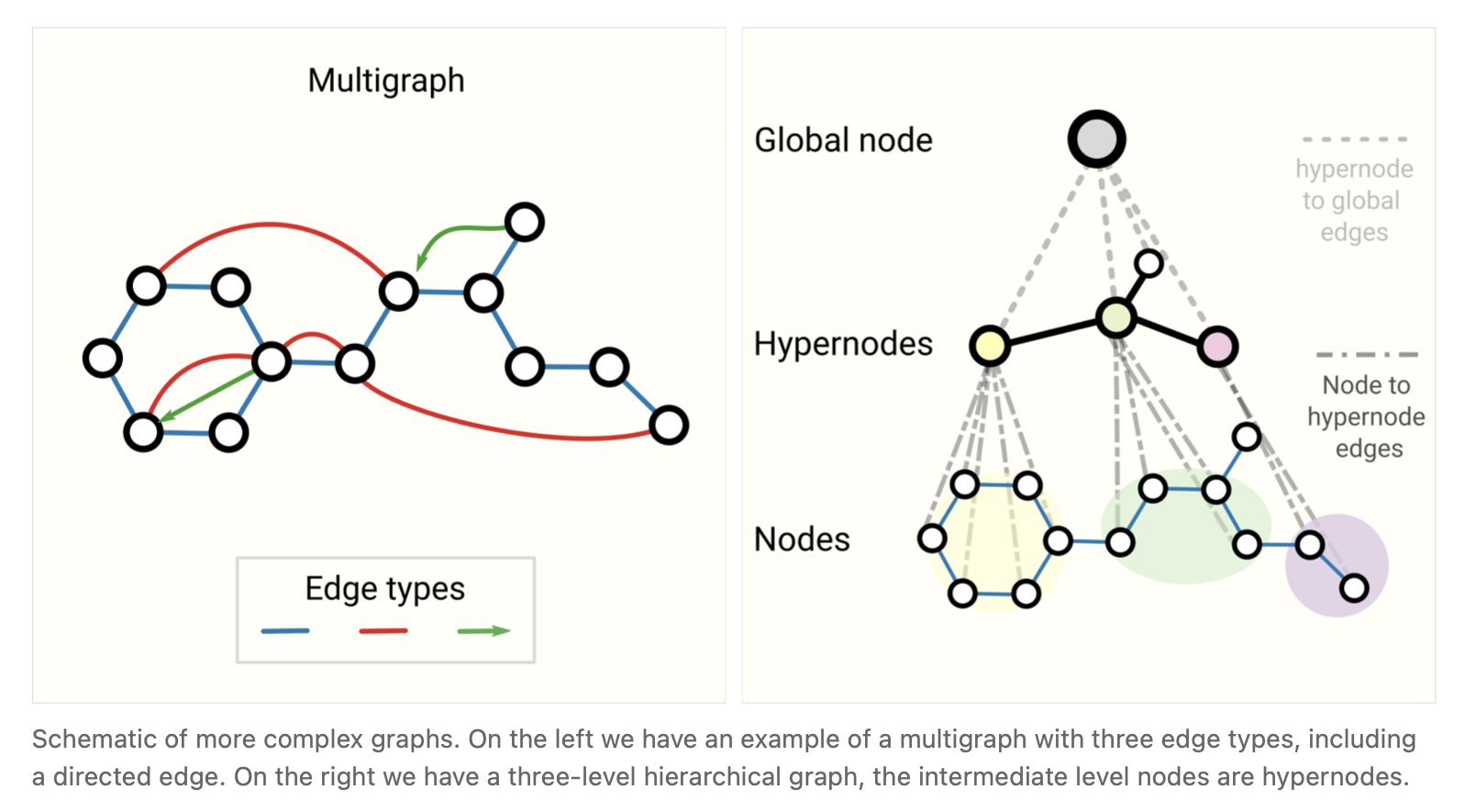
图1 一些复杂图的示意图。在左边,我们有一个多重图的例子,它有三种边类型,包括有向边。在右边我们有一个三层的层次图,中间层的节点是超节点。
How to train and design GNNs that have multiple types of graph attributes is a current area of research [37] , [38] .
如何训练和设计具有多种图属性类型的GNN是当前研究的一个领域,[37],[38]。
Sampling Graphs and Batching in GNNs
GNN中的采样图和批处理
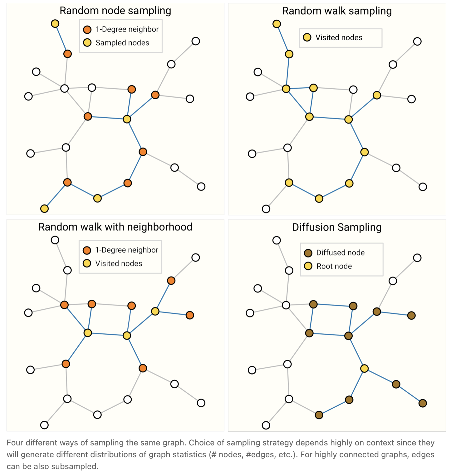
A common practice for training neural networks is to update network parameters with gradients calculated on randomized constant size (batch size) subsets of the training data (mini-batches). This practice presents a challenge for graphs due to the variability in the number of nodes and edges adjacent to each other, meaning that we cannot have a constant batch size. The main idea for batching with graphs is to create subgraphs that preserve essential properties of the larger graph. This graph sampling operation is highly dependent on context and involves sub-selecting nodes and edges from a graph. These operations might make sense in some contexts (citation networks) and in others, these might be too strong of an operation (molecules, where a subgraph simply represents a new, smaller molecule). How to sample a graph is an open research question. [39] If we care about preserving structure at a neighborhood level, one way would be to randomly sample a uniform number of nodes, our node-set. Then add neighboring nodes of distance k adjacent to the node-set, including their edges. [40] Each neighborhood can be considered an individual graph and a GNN can be trained on batches of these subgraphs. The loss can be masked to only consider the node-set since all neighboring nodes would have incomplete neighborhoods. A more efficient strategy might be to first randomly sample a single node, expand its neighborhood to distance k, and then pick the other node within the expanded set. These operations can be terminated once a certain amount of nodes, edges, or subgraphs are constructed. If the context allows, we can build constant size neighborhoods by picking an initial node-set and then sub-sampling a constant number of nodes (e.g randomly, or via a random walk or Metropolis algorithm [41] ).
训练神经网络的一种常见做法是用训练数据的随机常数大小(批量大小)子集(小批量)计算出的梯度来更新网络参数。由于相邻的节点和边的数量的可变性,这一实践给图带来了挑战,这意味着我们不能有一个恒定的批处理大小。对图进行批处理的主要思想是创建保留较大图的基本属性的子图。这种图采样操作高度依赖于上下文,涉及从图中选择子节点和边。这些操作可能在某些情况下(引用网络)是有意义的,而在其他情况下,这些操作可能过于强大(分子,其中一个子图只是表示一个新的、更小的分子)。如何对图表进行抽样是一个开放性的研究问题。[39] 如果我们想在邻域水平上保持结构,一种方法是随机抽样一个均匀数目的节点,我们的节点集。然后添加与节点集相邻的距离为k的相邻节点,包括它们的边。[40] 每个邻域可以被视为一个单独的图,并且可以在这些子图的批量上训练GNN。由于所有的邻近节点都有不完整的邻域,因此损失可以被掩盖,只考虑节点集。一个更有效的策略可能是,首先对单个节点进行随机抽样,将其邻域扩展到距离k,然后在扩展的集合中选择另一个节点。一旦构造了一定数量的节点、边或子图,这些操作就可以终止。如果环境允许,我们可以通过选择一个初始节点集,然后对一个恒定数量的节点进行子抽样(例如随机抽样,或通过随机遍历或Metropolis算法[41])来构建恒定大小的邻域。
有关其中一些采样方法法中如果小伙伴们不太懂可以参考 相关采样算法
Sampling a graph is particularly relevant when a graph is large enough that it cannot be fit in memory. Inspiring new architectures and training strategies such as Cluster-GCN [42] and GraphSaint [43] . We expect graph datasets to continue growing in size in the future.
当一个图大到无法装入内存时,对图进行采样尤为重要。启发新的架构和训练策略,如Cluster-GCN [42] 和GraphSaint [43]。我们预计未来图的数据集的规模将继续增长。
Inductive biases
归纳偏差
When building a model to solve a problem on a specific kind of data, we want to specialize our models to leverage the characteristics of that data. When this is done successfully, we often see better predictive performance, lower training time, fewer parameters and better generalization.
在构建模型以解决特定类型数据上的问题时,我们希望将模型特殊化,以适应该数据的特征。当这一点成功地完成时,我们通常会看到更好的预测性能,更低的训练时间,更少的参数和更好的泛化。
When labeling on images, for example, we want to take advantage of the fact that a dog is still a dog whether it is in the top-left or bottom-right corner of an image. Thus, most image models use convolutions, which are translation invariant. For text, the order of the tokens is highly important, so recurrent neural networks process data sequentially. Further, the presence of one token (e.g. the word ‘not’) can affect the meaning of the rest of a sentence, and so we need components that can ‘attend’ to other parts of the text, which transformer models like BERT and GPT-3 can do. These are some examples of inductive biases, where we are identifying symmetries or regularities in the data and adding modelling components that take advantage of these properties.
例如,当在图像上做标签时,我们希望利用这样一个事实,即无论在图像的左上角还是右下角,一只狗仍然是一只狗。因此,大多数图像模型使用卷积,因为它是平移不变的。对于文本,符号的顺序非常重要,因此循环神经网络适合处理顺序数据。此外,一个标记(例如单词“not”)的出现会影响句子其余部分的意思,因此我们需要能够“注意”文本其他部分的组成,这是像BERT和GPT-3这样的转换模型可以做到的。这是一些归纳偏差的例子,我们在其中识别数据中的对称性或规律性,并添加利用这些属性的建模组成部分。
In the case of graphs, we care about how each graph component (edge, node, global) is related to each other so we seek models that have a relational inductive bias. [19] A model should preserve explicit relationships between entities (adjacency matrix) and preserve graph symmetries (permutation invariance). We expect problems where the interaction between entities is important will benefit from a graph structure. Concretely, this means designing transformation on sets: the order of operation on nodes or edges should not matter and the operation should work on a variable number of inputs.
在图的情况下,我们关心每个图组件(边、节点、全局)是如何相互关联的,因此我们寻找具有关系归纳偏向的模型。[19] 模型应保持实体之间的显式关系(邻接矩阵),并保持图的对称性(置换不变性)。我们期望实体之间的交互很重要的问题将从图结构中受益。具体地说,这意味着在集合上设计变换: 节点或边的操作顺序不重要,操作可以在一个可变数量的输入上进行。
Comparing aggregation operations
比较聚合操作
Pooling information from neighboring nodes and edges is a critical step in any reasonably powerful GNN architecture. Because each node has a variable number of neighbors, and because we want a differentiable method of aggregating this information, we want to use a smooth aggregation operation that is invariant to node ordering and the number of nodes provided.
在任何功能相当强大的GNN模型结构中,集中来自邻近节点和边的信息都是一个关键步骤。由于每个节点的邻居数量是可变的,而且我们需要一种可微分的方法来聚合这些信息,因此我们希望使用一种平滑的聚合操作,该操作对节点顺序和所提供的节点数量是不变的。
Selecting and designing optimal aggregation operations is an open research topic. [44] A desirable property of an aggregation operation is that similar inputs provide similar aggregated outputs, and vice-versa. Some very simple candidate permutation-invariant operations are sum, mean, and max. Summary statistics like variance also work. All of these take a variable number of inputs, and provide an output that is the same, no matter the input ordering. Let’s explore the difference between these operations.
选择和设计最优聚合操作是一个开放的研究课题。[44] 聚合操作的一个理想属性是,类似的输入提供类似的聚合输出,反之亦然。一些非常简单的候选置换不变运算是和、均值和最大值。像方差这样的聚合方式也是可行的。无论输入顺序如何,所有这些都接受数量可变的输入,并提供相同的输出。让我们探讨一下这些操作之间的区别。
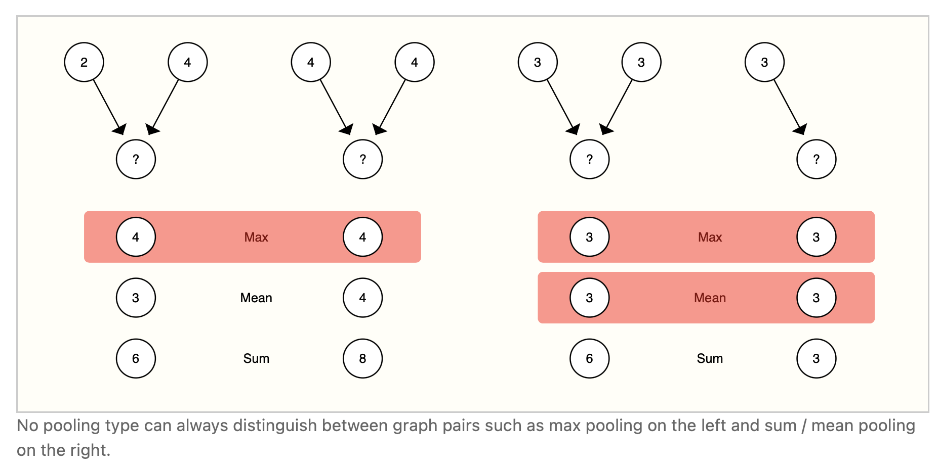
There is no operation that is uniformly the best choice. The mean operation can be useful when nodes have a highly-variable number of neighbors or you need a normalized view of the features of a local neighborhood. The max operation can be useful when you want to highlight single salient features in local neighborhoods. Sum provides a balance between these two, by providing a snapshot of the local distribution of features, but because it is not normalized, can also highlight outliers. In practice, sum is commonly used.
没有一种操作总是的最佳的选择。当节点的邻居数量高度可变时,或者需要对局部邻居的特征进行规范化处理时,mean操作非常有用。当您想要突出局部社区的单个显著特征时,max操作可能很有用。sum通过提供特性的局部分布的快照,在这两者之间提供了一种平衡,但是因为它不是标准化的,所以也可以突出显示离群值。在实践中,通常使用sum。
Designing aggregation operations is an open research problem that intersects with machine learning on sets. [45] New approaches such as Principal Neighborhood aggregation [27] take into account several aggregation operations by concatenating them and adding a scaling function that depends on the degree of connectivity of the entity to aggregate. Meanwhile, domain specific aggregation operations can also be designed. One example lies with the “Tetrahedral Chirality” aggregation operators [46] .
集合上的聚合操作设计是一个与机器学习交叉的开放研究问题。[45] 诸如Principal Neighborhood aggregation [27] 这样的新方法通过将这些聚合操作连接起来,并添加一个依赖于实体的连接性程度的扩展函数来考虑聚合操作。同时,还可以设计特定于领域的聚合操作。一个例子就是“Tetrahedral Chirality”聚集算子 [46]。
GCN as subgraph function approximators
GCN作为子图函数逼近器
Another way to see GCN (and MPNN) of k-layers with a 1-degree neighbor lookup is as a neural network that operates on learned embeddings of subgraphs of size k. [47] [44]
另一种观察k层的GCN(和MPNN)和距离为1度的邻居查找的方法是,将其作为一个神经网络,在大小为k的子图的学习embeddings中运行。[47] [44]
When focusing on one node, after k-layers, the updated node representation has a limited viewpoint of all neighbors up to k-distance, essentially a subgraph representation. Same is true for edge representations.
当聚焦于一个节点时,在k层之后,更新的节点表示具有到k距离为止所有邻居的有节点,本质上是一个子图表示。对于边的表示也是如此。
So a GCN is collecting all possible subgraphs of size k and learning vector representations from the vantage point of one node or edge. The number of possible subgraphs can grow combinatorially, so enumerating these subgraphs from the beginning vs building them dynamically as in a GCN, might be prohibitive.
所以GCN是收集所有大小为k的可能的子图,并从一个节点或边的有利位置进行向量表示。适合的子图数量可以组合式增长,所以如果不是像在GCN中那样动态地构建这些子图,而是从一开始就枚举它们,可能是行不通的。
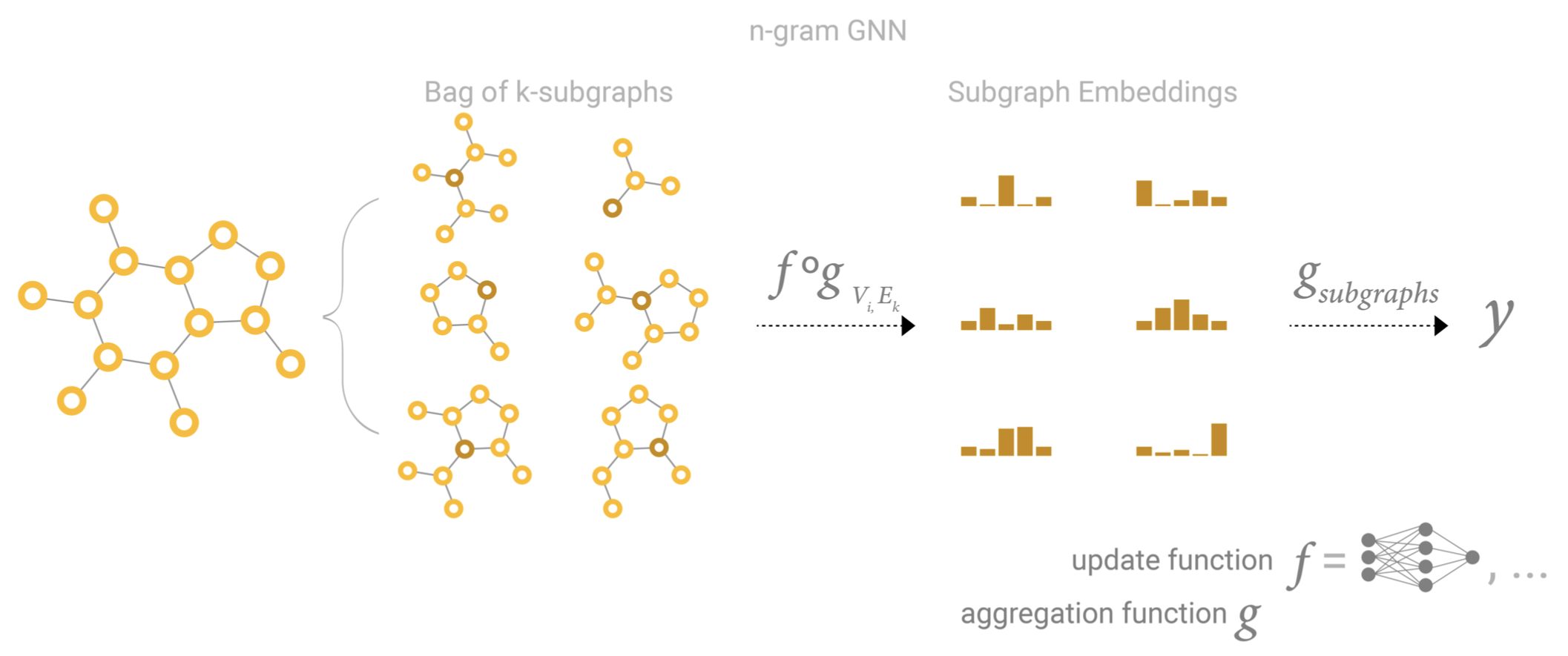 图4 n-gram GNN
Edges and the Graph Dual
边与图的对偶
One thing to note is that edge predictions and node predictions, while seemingly different, often reduce to the same problem: an edge prediction task on a graph G G G can be phrased as a node-level prediction on G G G’s dual.
需要注意的一点是,边的预测和节点预测虽然看起来不同,但往往归结为同一个问题: 图 G G G上的边层面的预测任务可以被描述为 G G G对偶的节点层面的预测。
To obtain G G G’s dual, we can convert nodes to edges (and edges to nodes). A graph and its dual contain the same information, just expressed in a different way. Sometimes this property makes solving problems easier in one representation than another, like frequencies in Fourier space. In short, to solve an edge classification problem on G G G, we can think about doing graph convolutions on G G G’s dual (which is the same as learning edge representations on G G G), this idea was developed with Dual-Primal Graph Convolutional Networks. [48]
为了得到 G G G的对偶,我们可以将节点转换为边(或将边转换为节点)。图及其对偶包含相同的信息,只是表示方式不同而已。有时,这个特性使得在一种表示法(节点的表示/边的表示)中解决问题比在另一种表示法中容易,比如傅里叶空间中的频率。简而言之,为了解决 G G G上的边的分类问题,我们可以考虑在 G G G的对偶上进行图卷积(这与在 G G G上学习边缘表示是一样的),这个想法是由Dual - Primal图卷积网络发展而来的。[48]
Graph convolutions as matrix multiplications, and matrix multiplications as walks on a graph
图的卷积是矩阵乘法,矩阵乘法是在图上游走
We’ve talked a lot about graph convolutions and message passing, and of course, this raises the question of how do we implement these operations in practice? For this section, we explore some of the properties of matrix multiplication, message passing, and its connection to traversing a graph.
我们已经讨论了很多关于图卷积和信息传递的内容,当然,这也出现了一个问题,即如何在实践中实现这些操作?在本节中,我们将探讨矩阵乘法的一些属性、信息传递以及它与遍历图的连接。
The first point we want to illustrate is that the matrix multiplication of an adjacent matrix A A A n n o d e s × n n o d e s n_{nodes}×n_{nodes} nnodes×nnodes with a node feature matrix {X} of size n n o d e s × n o d e d i m n_{nodes}×node_{dim} nnodes×nodedim implements an simple message passing with a summation aggregation. Let the matrix be B = A X B=AX B=AX, we can observe that any entry B i j B_{ij} Bij can be expressed as < A r o w i X ˙ c o l u m n j > = A i , 1 X 1 , j + A i , 2 X 2 , j + ⋯ + A i , n X n , j = ∑ A i , k > 0 X k , j <A_{row_i}\ \dot{X}_{column_j}>=A_{i,1} X_{1,j}+A_{i,2} X_{2,j}+⋯+A_{i,n} X_{n,j}=∑_{A_{i,k}>0}X_{k,j} <Arowi X˙columnj>=Ai,1X1,j+Ai,2X2,j+⋯+Ai,nXn,j=∑Ai,k>0Xk,j . Because A i , k A_{i,k} Ai,k
are binary entries only when a edge exists between n o d e i node_i nodei and n o d e j node_j nodej, the inner product is essentially “gathering” all node features values of dimension j j j” that share an edge with n o d e i node_i nodei. It should be noted that this message passing is not updating the representation of the node features, just pooling neighboring node features. But this can be easily adapted by passing X X X through your favorite differentiable transformation (e.g. MLP) before or after the matrix multiply.
我们想要说明的第一点是,大小为 n n o d e s × n n o d e s n_{nodes}×n_{nodes} nnodes×nnodes的邻接矩阵 A A A与大小为 n n o d e s × n o d e d i m n_{nodes}×node_{dim} nnodes×nodedim的节点特征矩阵X的矩阵乘法实现了一个简单的信息传递和聚合操作。设矩阵为 B = A X B=AX B=AX,可以看到任意项 B i j B_{ij} Bij都可以表示为 < A r o w i X ˙ c o l u m n j > = A i , 1 X 1 , j + A i , 2 X 2 , j + ⋯ + A i , n X n , j = ∑ A i , k > 0 X k , j <A_{row_i}\ \dot{X}_{column_j}>=A_{i,1} X_{1,j}+A_{i,2} X_{2,j}+⋯+A_{i,n} X_{n,j}=∑_{A_{i,k}>0}X_{k,j} <Arowi X˙columnj>=Ai,1X1,j+Ai,2X2,j+⋯+Ai,nXn,j=∑Ai,k>0Xk,j 。因为只有当节点 i i i和节点 k k k之间存在一条边时, A i , k A_{i,k} Ai,k才是二进制项,所以内积本质上是“收集”与 n o d e i node_i nodei共享一条边的维数为j的所有节点特征值。值得注意的是,这个信息传递并不是更新节点特征的表示方法,只是对邻近节点的特征进行了池化操作。但是在矩阵乘法之前或之后通过合适于你的可微变换(例如MLP)传递 X X X可以很容易地进行调整。
From this view, we can appreciate the benefit of using adjacency lists. Due to the expected sparsity of A A A we don’t have to sum all values where A i , j A_{i,j} Ai,j is zero. As long as we have an operation to gather values based on an index, we should be able to just retrieve positive entries. Additionally, this matrix multiply-free approach frees us from using summation as an aggregation operation.
从这个角度来看,我们可以体会到使用邻接表的好处。由于 A A A的期望稀疏性我们不需要对所有 A i , j A_{i,j} Ai,j为0的值求和。只要我们有一个基于索引收集值的操作,我们就应该能够检索正(大于0)的条目。此外,这种无需矩阵乘法的方法使我们不必将求和作为聚合操作来使用。
We can imagine that applying this operation multiple times allows us to propagate information at greater distances. In this sense, matrix multiplication is a form of traversing over a graph. This relationship is also apparent when we look at powers A K A^K AK of the adjacency matrix. If we consider the matrix A 2 A^2 A2, the term A i j 2 A_{ij}^2 Aij2 counts all walks of length 2 from n o d e i node_i nodei to n o d e j node_j nodej and can be expressed as the inner product < A r o w i , A c o l u m n j > = A i , 1 A 1 , j + A i , 2 A 2 , j + ⋯ + A i , n A n , j <A_{row_i}, A_{column_j}>=A_{i,1} A_{1,j}+A_{i,2} A_{2,j}+⋯+A_{i,n} A_{n,j} <Arowi,Acolumnj>=Ai,1A1,j+Ai,2A2,j+⋯+Ai,nAn,j. The intuition is that the first term a i , 1 a_{i,1} ai,1 a 1 , j a_{1,j} a1,j is only positive under two conditions, there is edge that connects n o d e i node_i nodei to n o d e 1 node_1 node1 and another edge that connects n o d e 1 node_1 node1 to n o d e j node_j nodej . In other words, both edges form a path of length 2 that goes from n o d e i node_i nodei to n o d e j node_j nodej passing by n o d e 1 node_1 node1. Due to the summation, we are counting over all possible intermediate nodes. This intuition carries over when we consider A 3 = A A 2 A^3=AA^2 A3=AA2 … and so on to A k A^k Ak.
我们可以想象,多次应用这个操作可以让我们在更大的距离上传递信息。从这个意义上说,矩阵乘法是遍历图的一种形式。当我们看邻接矩阵的 A K A^K AK时,这种关系也很明显。如果我们考虑矩阵 A 2 A^2 A2,项 A i j 2 A_{ij}^2 Aij2计算从节点i到节点 j j j所有长度为2的步长,可以表示为内积 < A r o w i , A c o l u m n j > = A i , 1 A 1 , j + A i , 2 A 2 , j + ⋯ + A i , n A n , j <A_{row_i}, A_{column_j}>=A_{i,1} A_{1,j}+A_{i,2} A_{2,j}+⋯+A_{i,n} A_{n,j} <Arowi,Acolumnj>=Ai,1A1,j+Ai,2A2,j+⋯+Ai,nAn,j。直觉告诉我们第一项 a i , 1 a_{i,1} ai,1 a 1 , j a_{1,j} a1,j只有在两种情况下是正的,有一条边连接着 n o d e i node_i nodei和 n o d e 1 node_1 node1,另一条边连接着 n o d e 1 node_1 node1和 n o d e j node_j nodej。换句话说,两条边的长度都是2,从 n o d e i node_i nodei到 n o d e j node_j nodej经过 n o d e 1 node_1 node1,由于求和,我们在计算所有可能的中间节点。当我们考虑 A 3 = A A 2 A^3=AA^2 A3=AA2…一直到 A k A^k Ak,这种直觉依然有效。
There are deeper connections on how we can view matrices as graphs to explore [49] [50] [51] .
在如何将矩阵视为图进行探索方面,还有更深层次的联系[49] [50] [51]。
Graph Attention Networks
图注意力网络
Another way of communicating information between graph attributes is via attention. [52] For example, when we consider the sum-aggregation of a node and its 1-degree neighboring nodes we could also consider using a weighted sum.The challenge then is to associate weights in a permutation invariant fashion. One approach is to consider a scalar scoring function that assigns weights based on pairs of nodes ( f ( n o d e i , n o d e j ) f(node_i,node_j) f(nodei,nodej)). In this case, the scoring function can be interpreted as a function that measures how relevant a neighboring node is in relation to the center node. Weights can be normalized, for example with a softmax function to focus most of the weight on a neighbor most relevant for a node in relation to a task. This concept is the basis of Graph Attention Networks (GAT) [53] and Set Transformers [54] . Permutation invariance is preserved, because scoring works on pairs of nodes. A common scoring function is the inner product and nodes are often transformed before scoring into query and key vectors via a linear map to increase the expressivity of the scoring mechanism. Additionally for interpretability, the scoring weights can be used as a measure of the importance of an edge in relation to a task.
图属性之间传递信息的另一种方式是通过注意力[52]。例如,当我们考虑一个节点及其1次邻近节点的sum聚合操作时,我们也可以考虑使用加权和。那么,其带来的挑战就是以一种置换不变的方式关联权重。一种方法是考虑一个标量评分函数,根据节点( f ( n o d e i , n o d e j ) f(node_i,node_j) f(nodei,nodej))分配权重。在这种情况下,评分函数可以被解释为一个用来衡量一个相邻节点与中心节点之间相关性的函数。权重可以归一化,例如使用softmax函数,将权重的大部分集中在与任务相关的节点最相关的邻居上。这个概念是图注意力网络(GAT) [53] 和设置Transformers [54] 的基础。排列不变性被保留,因为评分工作对节点。常用的评分函数是内积,评分前通常通过线性映射将节点转换为查询和关键向量,以增加评分机制的表达力。此外,对于可解释性,评分权重可以用来衡量与任务相关优势的重要性。
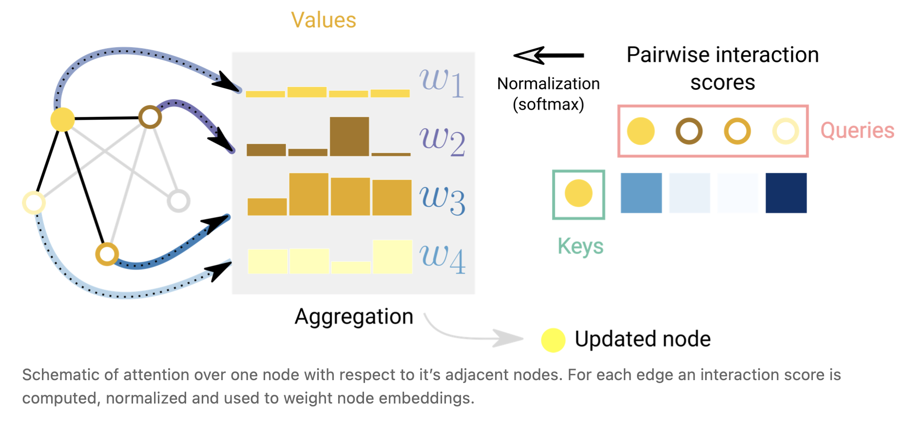 图5 一个节点相对于相邻节点的注意力示意图。对每条边计算、归一化并用于加权节点embeddings。
Additionally, transformers can be viewed as GNNs with an attention mechanism [55] . Under this view, the transformer models several elements (i.g. character tokens) as nodes in a fully connected graph and the attention mechanism is assigning edge embeddings to each node-pair which are used to compute attention weights. The difference lies in the assumed pattern of connectivity between entities, a GNN is assuming a sparse pattern and the Transformer is modelling all connections.
此外,transformers可以看作是具有注意力机制的GNN [55] 。在这种观点下,变压器将几个元素(例如字符标记)建模为一个全连通图中的节点,注意力机制是为每个节点对分配边embeddings,这些节点对用于计算注意权重。不同之处在于实体之间连接的假设模式,GNN假设稀疏模式,Transformer对所有连接建模。
Graph explanations and attributions
图的解释性和attribution技术
When deploying GNN in the wild we might care about model interpretability for building credibility, debugging or scientific discovery. The graph concepts that we care to explain vary from context to context. For example, with molecules we might care about the presence or absence of particular subgraphs [56] , while in a citation network we might care about the degree of connectedness of an article. Due to the variety of graph concepts, there are many ways to build explanations. GNNExplainer [57] casts this problem as extracting the most relevant subgraph that is important for a task. Attribution techniques [58] assign ranked importance values to parts of a graph that are relevant for a task. Because realistic and challenging graph problems can be generated synthetically, GNNs can serve as a rigorous and repeatable testbed for evaluating attribution techniques [59] .
在部署GNN模型时,我们可能会关心模型的可解释性,以建立可信性、调试或科学发现。我们要解释的图概念因上下文的不同而不同。例如,对于分子,我们可能关心特定子图的存在与否[56],而在引文网络中,我们可能关心文章的连通性程度。由于图概念的多样性,有许多方法来构建解释。GNNExplainer [57]将此问题转换为提取对任务至关重要的最相关的子图。Attribution技术[58]将排序的重要性值分配给图中与任务相关的部分。由于可以综合生成现实且具有挑战性的图问题,因此GNN可以作为评估attribution技术的严格且可重复的测试平台[59]。
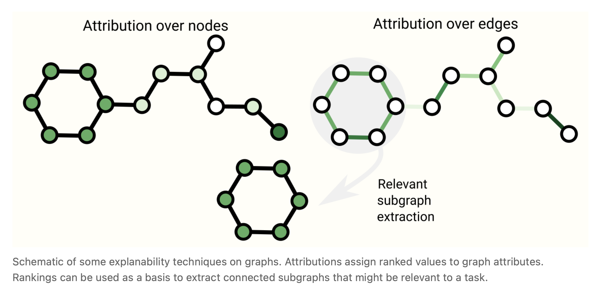 图6 图的一些可解释技术的示意图。属性将排序的值分配给图属性。排名可以作为提取可能与任务相关的连接子图的基础。
Generative modelling
生成模型
Besides learning predictive models on graphs, we might also care about learning a generative model for graphs. With a generative model we can generate new graphs by sampling from a learned distribution or by completing a graph given a starting point. A relevant application is in the design of new drugs, where novel molecular graphs with specific properties are desired as candidates to treat a disease.
除了学习图上的预测模型之外,我们还可能关心学习图的生成模型。在生成模型中,我们可以通过从一个学习过的分布中抽样或通过给定一个起点完成一个图来生成新的图。一个相关的应用是在新药的设计中,需要具有特定特性的新型分子图作为治疗疾病的备选。
A key challenge with graph generative models lies in modelling the topology of a graph, which can vary dramatically in size and has N n o d e s 2 N_{nodes}^2 Nnodes2 terms. One solution lies in modelling the adjacency matrix directly like an image with an autoencoder framework. [60] The prediction of the presence or absence of an edge is treated as a binary classification task. The N n o d e s 2 N_{nodes}^2 Nnodes2 term can be avoided by only predicting known edges and a subset of the edges that are not present. The graphVAE learns to model positive patterns of connectivity and some patterns of non-connectivity in the adjacency matrix.
图的生成模型的一个关键挑战是对图的拓扑结构进行建模,图的拓扑结构大小可以有很大的变化,并且有 N n o d e s 2 N_{nodes}^2 Nnodes2个项。一种解决方案是直接像使用自动编码器框架的图像一样建模邻接矩阵[60]。对边存在与否的预测被视为一项二元分类任务。 N n o d e s 2 N_{nodes}^2 Nnodes2项可以通过只预测已知边和不存在边的子集来避免。graphVAE学习建模邻接矩阵中连接的正模式和一些非连接的模式。
Another approach is to build a graph sequentially, by starting with a graph and applying discrete actions such as addition or subtraction of nodes and edges iteratively. To avoid estimating a gradient for discrete actions we can use a policy gradient. This has been done via an auto-regressive model, such a RNN [61] , or in a reinforcement learning scenario. [62] Furthermore, sometimes graphs can be modeled as just sequences with grammar elements. [63] [64]
另一种方法是按顺序构建图,从图开始,迭代地应用离散操作(如节点和边的加法或减法)。为了避免估计离散动作的梯度,我们可以使用策略梯度。这是通过自回归模型,如RNN [61],或在强化学习场景中完成的[62]。此外,有时可以将图建模为带有语法元素的序列。[63] [64]
Final thoughts
总结与思考
Graphs are a powerful and rich structured data type that have strengths and challenges that are very different from those of images and text. In this article, we have outlined some of the milestones that researchers have come up with in building neural network based models that process graphs. We have walked through some of the important design choices that must be made when using these architectures, and hopefully the GNN playground can give an intuition on what the empirical results of these design choices are. The success of GNNs in recent years creates a great opportunity for a wide range of new problems, and we are excited to see what the field will bring.
图是一种功能强大且丰富的结构化数据类型,它的优势和挑战与图像和文本非常不同。在本文中,我们概述了研究人员在构建基于处理图形的神经网络模型时所提出的一些里程碑。我们已经讨论了在使用这些架构时必须做出的一些重要设计选择,希望GNN playground能够直观地了解这些设计选择的经验结果是什么。近年来GNN的成功为一系列新问题创造了巨大的机遇,我们很高兴看到该领域将带来什么。
参考文献
[19] Relational inductive biases, deep learning, and graph networks Battaglia, P.W., Hamrick, J.B., Bapst, V., Sanchez-Gonzalez, A., Zambaldi, V., Malinowski, M., Tacchetti, A., Raposo, D., Santoro, A., Faulkner, R., Gulcehre, C., Song, F., Ballard, A., Gilmer, J., Dahl, G., Vaswani, A., Allen, K., Nash, C., Langston, V., Dyer, C., Heess, N., Wierstra, D., Kohli, P., Botvinick, M., Vinyals, O., Li, Y. and Pascanu, R., 2018.
[27] Principal Neighbourhood Aggregation for Graph Nets Corso, G., Cavalleri, L., Beaini, D., Lio, P. and Velickovic, P., 2020.
[32] Graph Theory Harary, F., 1969.
[33] A nested-graph model for the representation and manipulation of complex objects Poulovassilis, A. and Levene, M., 1994. ACM Transactions on Information Systems, Vol 12(1), pp. 35--68.
[34] Modeling polypharmacy side effects with graph convolutional networks Zitnik, M., Agrawal, M. and Leskovec, J., 2018. Bioinformatics, Vol 34(13), pp. i457--i466.
[35] Machine learning in chemical reaction space Stocker, S., Csanyi, G., Reuter, K. and Margraf, J.T., 2020. Nat. Commun., Vol 11(1), pp. 5505.
[36] Graphs and Hypergraphs Berge, C., 1976. Elsevier.
[37] HyperGCN: A New Method of Training Graph Convolutional Networks on Hypergraphs Yadati, N., Nimishakavi, M., Yadav, P., Nitin, V., Louis, A. and Talukdar, P., 2018.
[38] Hierarchical Message-Passing Graph Neural Networks Zhong, Z., Li, C. and Pang, J., 2020.
[39] Little Ball of Fur Rozemberczki, B., Kiss, O. and Sarkar, R., 2020. Proceedings of the 29th ACM International Conference on Information & Knowledge Management.
[40] Sampling from large graphs Leskovec, J. and Faloutsos, C., 2006. Proceedings of the 12th ACM SIGKDD international conference on Knowledge discovery and data mining - KDD '06.
[41] Metropolis Algorithms for Representative Subgraph Sampling Hubler, C., Kriegel, H., Borgwardt, K. and Ghahramani, Z., 2008. 2008 Eighth IEEE International Conference on Data Mining.
[42] Cluster-GCN: An Efficient Algorithm for Training Deep and Large Graph Convolutional Networks Chiang, W., Liu, X., Si, S., Li, Y., Bengio, S. and Hsieh, C., 2019.
[43] GraphSAINT: Graph Sampling Based Inductive Learning Method Zeng, H., Zhou, H., Srivastava, A., Kannan, R. and Prasanna, V., 2019.
[44] How Powerful are Graph Neural Networks? Xu, K., Hu, W., Leskovec, J. and Jegelka, S., 2018.
[45] Rep the Set: Neural Networks for Learning Set Representations Skianis, K., Nikolentzos, G., Limnios, S. and Vazirgiannis, M., 2019.
[46] Message Passing Networks for Molecules with Tetrahedral Chirality Pattanaik, L., Ganea, O., Coley, I., Jensen, K.F., Green, W.H. and Coley, C.W., 2020.
[47] N-Gram Graph: Simple Unsupervised Representation for Graphs, with Applications to Molecules Liu, S., Demirel, M.F. and Liang, Y., 2018.
[48] Dual-Primal Graph Convolutional Networks Monti, F., Shchur, O., Bojchevski, A., Litany, O., Gunnemann, S. and Bronstein, M.M., 2018.
[49] Viewing matrices & probability as graphs Bradley, T..
[50] Graphs and Matrices Bapat, R.B., 2014. Springer.
[51] Modern Graph Theory Bollobas, B., 2013. Springer Science & Business Media.
[52] Attention Is All You Need Vaswani, A., Shazeer, N., Parmar, N., Uszkoreit, J., Jones, L., Gomez, A.N., Kaiser, L. and Polosukhin, I., 2017.
[53] Graph Attention Networks Velickovic, P., Cucurull, G., Casanova, A., Romero, A., Lio, P. and Bengio, Y., 2017.
[54] Set Transformer: A Framework for Attention-based Permutation-Invariant Neural Networks Lee, J., Lee, Y., Kim, J., Kosiorek, A.R., Choi, S. and Teh, Y.W., 2018.
[55] Transformers are Graph Neural Networks Joshi, C., 2020. NTU Graph Deep Learning Lab.
[56] Using Attribution to Decode Dataset Bias in Neural Network Models for Chemistry McCloskey, K., Taly, A., Monti, F., Brenner, M.P. and Colwell, L., 2018.
[57] GNNExplainer: Generating Explanations for Graph Neural Networks Ying, Z., Bourgeois, D., You, J., Zitnik, M. and Leskovec, J., 2019. Advances in Neural Information Processing Systems, Vol 32, pp. 9244--9255. Curran Associates, Inc.
[58] Explainability Methods for Graph Convolutional Neural Networks Pope, P.E., Kolouri, S., Rostami, M., Martin, C.E. and Hoffmann, H., 2019. 2019 IEEE/CVF Conference on Computer Vision and Pattern Recognition (CVPR).
[59] Evaluating Attribution for Graph Neural Networks Sanchez-Lengeling, B., Wei, J., Lee, B., Reif, E., Qian, W., Wang, Y., McCloskey, K.J., Colwell, L. and Wiltschko, A.B., 2020. Advances in Neural Information Processing Systems 33.
[60] Variational Graph Auto-Encoders Kipf, T.N. and Welling, M., 2016.
[61] GraphRNN: Generating Realistic Graphs with Deep Auto-regressive Models You, J., Ying, R., Ren, X., Hamilton, W.L. and Leskovec, J., 2018.
[62] Optimization of Molecules via Deep Reinforcement Learning Zhou, Z., Kearnes, S., Li, L., Zare, R.N. and Riley, P., 2019. Sci. Rep., Vol 9(1), pp. 1--10. Nature Publishing Group.
[63] Self-Referencing Embedded Strings (SELFIES): A 100% robust molecular string representation Krenn, M., Hase, F., Nigam, A., Friederich, P. and Aspuru-Guzik, A., 2019.
[64] GraphGen: A Scalable Approach to Domain-agnostic Labeled Graph Generation Goyal, N., Jain, H.V. and Ranu, S., 2020.
Citation
For attribution in academic contexts, please cite this work as
Sanchez-Lengeling, et al., "A Gentle Introduction to Graph Neural Networks", Distill, 2021.
BibTeX citation
@article{sanchez-lengeling2021a,
  author = {Sanchez-Lengeling, Benjamin and Reif, Emily and Pearce, Adam and Wiltschko, Alexander B.},
  title = {A Gentle Introduction to Graph Neural Networks},
  journal = {Distill},
  year = {2021},
  note = {https://distill.pub/2021/gnn-intro},
  doi = {10.23915/distill.00033}
}