多项式回归定义公式及案例
1、前言
之前写了一元和多元线性回归用来描述线性问题
机器学习:利用sklearn方法的一元线性回归模型(通过成绩预测绩点)_天海一直在的博客-CSDN博客_sklearn一元线性回归
机器学习:利用sklearn方法的多元线性回归模型(通过成绩预测绩点)_天海一直在的博客-CSDN博客_线性回归预测成绩
但如果我们找的不是直线或者超平面,而是一条曲线,那么就可以用多项式回归来分析和预测。
2、定义及公式
多项式回归可以写成:
Y i = β 0 + β 1 X i + β 2 X i 2 + . . . + β k X i k Y_{i} = \beta_{0} +\beta_{1}X_{i}+\beta_{2}X_{i}^2+...+\beta_{k}X_{i}^k Yi=β0+β1Xi+β2Xi2+...+βkXik
例如二次曲线:
y = a t 2 + b t + c y=at^2+bt+c y=at2+bt+c
3、案例代码
1、数据解析
首先有数据2020年2月24日至2020年4月30日疫情每日新增病例数和道琼斯指数,数据如下。
| date | new_cases | volume |
|---|---|---|
| 2020/2/24 | 2346 | 399452730 |
| 2020/2/25 | 2668 | 449962408 |
| 2020/2/26 | 3064 | 408252788 |
| 2020/2/27 | 4327 | 568873667 |
| 2020/2/28 | 4487 | 796064921 |
| 2020/3/2 | 6430 | 554364655 |
| 2020/3/3 | 8440 | 552440168 |
| 2020/3/4 | 7920 | 401575883 |
| 2020/3/5 | 9798 | 401427499 |
| 2020/3/6 | 13360 | 507343739 |
| 2020/3/9 | 15520 | 629729505 |
| 2020/3/10 | 17552 | 555995247 |
| 2020/3/11 | 27846 | 550900431 |
| 2020/3/12 | 21923 | 777537526 |
| 2020/3/13 | 52553 | 728758617 |
| 2020/3/16 | 54676 | 681933454 |
| 2020/3/17 | 58444 | 703490970 |
| 2020/3/18 | 71579 | 757446929 |
| 2020/3/19 | 98881 | 677652753 |
| 2020/3/20 | 110981 | 746325491 |
| 2020/3/23 | 151590 | 694579371 |
| 2020/3/24 | 144168 | 701764913 |
| 2020/3/25 | 180691 | 698482135 |
| 2020/3/26 | 220423 | 613646149 |
| 2020/3/27 | 225788 | 498053291 |
| 2020/3/30 | 222071 | 475736601 |
| 2020/3/31 | 262115 | 507392584 |
| 2020/4/1 | 275848 | 441398052 |
| 2020/4/2 | 277356 | 440119768 |
| 2020/4/3 | 283024 | 358248473 |
| 2020/4/6 | 241421 | 512454039 |
| 2020/4/7 | 237964 | 499183085 |
| 2020/4/8 | 276586 | 399118977 |
| 2020/4/9 | 284948 | 462544792 |
| 2020/4/13 | 230474 | 338246109 |
| 2020/4/14 | 279820 | 427996199 |
| 2020/4/15 | 257846 | 375498608 |
| 2020/4/16 | 316447 | 416772131 |
| 2020/4/17 | 284802 | 458032076 |
| 2020/4/20 | 240897 | 358856528 |
| 2020/4/21 | 242502 | 420993963 |
| 2020/4/22 | 263142 | 306933373 |
| 2020/4/23 | 268410 | 334639614 |
| 2020/4/24 | 293886 | 333127761 |
| 2020/4/27 | 223849 | 337304670 |
| 2020/4/28 | 238705 | 340993299 |
| 2020/4/29 | 247023 | 396245166 |
| 2020/4/30 | 260239 | 416383852 |
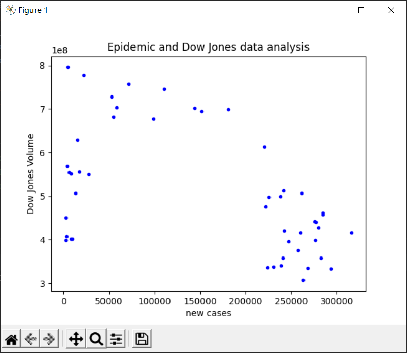
2、绘制散点图
对于该数据我们通过绘制散点图可以看出,这是一个多项式回归的模型
import matplotlib.pyplot as plt
import xlrd
import numpy as np
# 载入数据,打开excel文件
ExcelFile = xlrd.open_workbook("sandian.xls")
sheet1 = ExcelFile.sheet_by_index(0)
x = sheet1.col_values(0)
y = sheet1.col_values(1)
# 将列表转换为matrix
x = np.matrix(x).reshape(48, 1)
y = np.matrix(y).reshape(48, 1)

# 划线y
plt.title("Epidemic and Dow Jones data analysis")
plt.xlabel("new cases")
plt.ylabel("Dow Jones Volume")
plt.plot(x, y, 'b.')
plt.show()
3、多项式回归、拟合
通过散点图的趋势,我们选择拟合3次来防止过拟合和欠拟合。
import matplotlib.pyplot as plt
import numpy as np
import pandas as pd
from sklearn.metrics import r2_score
from matplotlib.font_manager import FontProperties  # 导入FontProperties

font = FontProperties(fname="SimHei.ttf", size=14)  # 设置字体

x = pd.read_excel('last_data.xls')['new_cases']
y = pd.read_excel('last_data.xls')['volume']

# 进行多项式拟合(这里选取3次多项式拟合)
z = np.polyfit(x, y, 3) # 用3次多项式拟合

# 获取拟合后的多项式
p = np.poly1d(z)
print(p)  # 在屏幕上打印拟合多项式

# 计算拟合后的y值
yvals=p(x)

# 计算拟合后的R方,进行检测拟合效果
r2 = r2_score(y, yvals)
print('多项式拟合R方为:', r2)

# 计算拟合多项式的极值点。
peak = np.polyder(p, 1)
print(peak.r)

# 画图对比分析
plot1 = plt.plot(x, y, '*', label='original values', color='red')
plot2 = plt.plot(x, yvals, '-', label='fitting values', color='blue',linewidth=2)

plt.xlabel('new_cases',fontsize=13, fontproperties=font)
plt.ylabel('Dow Jones Volume',fontsize=13, fontproperties=font)
plt.legend(loc="best")
plt.title('fitting diagram')
plt.show()
最后结果如下图
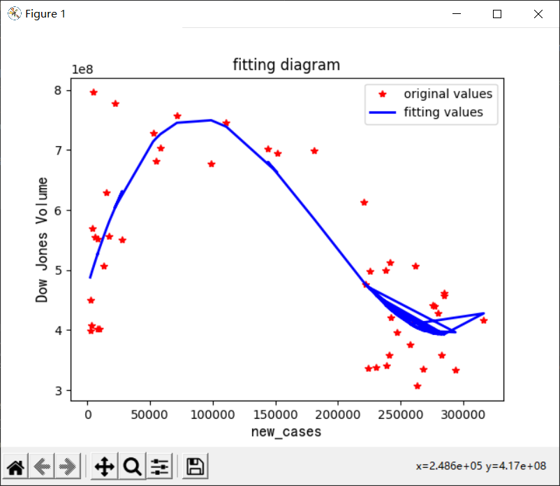
输出公式:
9.631e-08 x - 0.05356 x + 7169 x + 4.713e+08
多项式拟合R方为: 0.6462955787806361
[283148.64883622  87629.61932583]