python逻辑回归（logistic regression LR) 底层代码实现 BGD梯度下降算法 softmax多分类

逻辑回归

前面用sigmoid函数实现了基本逻辑回归的二分类，感兴趣的童鞋点击###python逻辑回归（logistic regression LR) 底层代码实现 BGD梯度下降算法 二分类#####了解sigmoid二分类逻辑回归

---

>>

---

前言

逻辑回归模型（Logistic Regression Model）是机器学习领域著名的分类模型。其常用于解决二分类（Binary Classification）问题。

但是在现实工作/学习/项目中，我们要解决的问题是经常多分类（Multiclass Classification）问题。

因此，需要对普通的基于sigmoid函数的逻辑回归模型进行拓展。本文介绍了 2 种拓展逻辑回归使其成为多分类模型的方法。

---

一、多0-1分类器

多0-1分类器是根据类别数建立多个0-1二分类器，主要有两种思路：One v One(OVO)和One v Rest（OVR)。

1.OVO

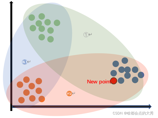
One-Vs-One 是一种相对稳健的扩展方法。对于多分类问题，假设类别数为C，让不同类别两两组合训练二分类模型，这样总共产生$C_C^2$组合，即$C_C^2$个分类器。

举例说明：如下图所示，假设待分类数为3,则应训练3个二分类器①（绿色椭圆）、②（红色椭圆）、③（蓝色椭圆）。对于图中new point，分别使用这三个分类器预测其类别，分类器①结果为蓝色类，分类器②结果为蓝色类，分类器③结果为红色类或绿色类（此结果不重要），所以三个分类器的分类结果为2蓝一红（或绿），此预测过程就像投票一样，得票数最多的为最终结果，所以红色点应属于蓝色类。

2.OVR

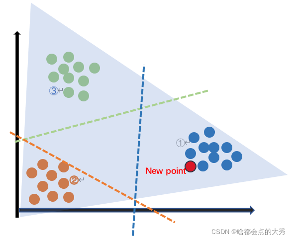
One v Rest（或者叫 One-Vs-All）转变的思路就如同方法名称描述的那样，选择其中一个类别为正类（Positive），使其他所有类别为负类（Negative）。

n 种类型的样本进行分类时，分别取一种样本作为一类，将剩余的所有类型的样本看做另一类，这样就形成了 n 个二分类问题，使用逻辑回归算法对 n 个数据集训练出 n 个模型，将待预测的样本传入这 n 个模型中，所得概率最高的那个模型对应的样本类型即认为是该预测样本的类型。
举例说明：分别已三角形顶点区域为正类，两底点区域所属的两类别为负类训练二分类模型，得到三个二分类器。对于图中new point，分别使用这三个分类器预测其类别，分类器①结果为蓝色类，分类器②结果为非绿色类（将蓝色类合红色类归于一类，分类器不清楚具体new point 属于哪一类），分类器③结果为非红色类（同上，分类器不清楚new point 属于蓝色类还是绿色类），一共有三个类，结果非绿非红，所以new point理所当然属于蓝色类。

3 OvO vs OvR：

OvO 用时较多，但其分类结果更准确，因为每一次二分类时都用真实的类型进行比较，没有混淆其它的类别。

二、softmax多分类

softmax函数

softmax函数可以将多分类的输出值转化为范围在[0,1]之间，和为1的概率分布。

$$softmax\left({\mathrm{Z}}_{\mathrm{i}}\right)=\frac{{\mathrm{e}}^{{\mathrm{Z}}_{\mathrm{i}}}}{{\sum }_{\mathrm{j}=1}^{\mathrm{C}}{\mathrm{e}}^{{\mathrm{Z}}_{\mathrm{j}}}}$$
其中,C为类别数，$Z_i$为样本经第i个分类器的输出值,i=1,2,3,…,C
$${\mathrm{Z}}_{\mathrm{i}}={\theta }_{\mathrm{i}}^{\mathrm{T}}\mathrm{X}$$
所以$$\mathrm{Z}={\theta }^{T}X=\left[\begin{array}{c}{\theta }_1^T\\ ⋮\\ {\theta }_C^T\end{array}\right]\cdot X=\left[\begin{array}{l}\left[{\theta }_1^0{\theta }_1^1{\theta }_1^2\cdots {\theta }_1^n\right]\\ ⋮\\ \left[{\theta }_C^0{\theta }_C^1{\theta }_C^2\cdots {\theta }_C^n\right]\end{array}\right]\cdot \left[\begin{array}{c}{x}_0\\ ⋮\\ x_{m+1}\end{array}\right]=\left[\begin{array}{c}{z}_0\\ ⋮\\ z_{m+1}\end{array}\right]$$

预测函数

预测函数选出数据经分类器后输出概率值的最大值所属类别，表达式如下：
$$h\left(Z\right)=arg\max \left(soft\max \left(Z\right)\right)=arg\max \left(soft\max \left(\left[Z_1,Z_2,\cdots ,Z_c\right]\right)\right)$$

损失函数

这里不对损失函数及其导数的关系式进行推导，感兴趣的童鞋可以去这里学习公式推导过程。
损失函数使用交叉熵函数,定义$$p_i=soft\max \left(Z_i\right)$$
于是
$$J\left(Z_j\right)=-\frac{1}{m}\sum _{i=1}^m\sum _{j=1}^C{y}_j^{\left(i\right)}\log \left(p_j^{\left(i\right)}\right)$$
其中，$y_j^{\left(i\right)}$为将y值进行one-hot编码后的值，表示第i个样本种第j列对应的值。

参数$\theta$对损失函数的导数关系

根据资料,$$\frac{\partial J}{\partial Z_j}=\left(p_j-y_j\right)$$

根据求导的链式法则，$$\frac{\partial J}{\partial \theta }=\frac{\partial J}{\partial Z}\cdot \frac{\partial Z}{\partial \theta }$$
所以，
$$\frac{\partial J}{\partial {\theta }_j^l}=\left(p_j-y_j\right)\cdot \frac{\partial Z}{\partial {\theta }_j^l}=\left(p_j-y_j\right)\cdot X^l$$
其中，${\theta }_j^l$为第j个分类器对应的第l个参数，参数更新公式完成。

softmax多分类逻辑回归底层代码实现及可视化

这里不对OVO和OVR方法进行编程，其代码原理较简单，只对SOFTMAX方法对应的逻辑回归进行编程及可视化。

import numpy as np
import pandas as pd
from sklearn.model_selection import train_test_split
from sklearn.datasets import make_blobs
import matplotlib.pyplot as plt
import matplotlib as mpl
from sklearn.metrics import confusion_matrix


def softmax(x,theta):#softmax假设函数
    p=[]
    for i in range(len(x)):
            p.append(np.power(np.e,np.dot(theta,x[i]))/np.sum(np.power(np.e,np.dot(theta,x[i]))))
    return np.array(p)

def LR_predict(x,theta,c1):#预测函数
    return np.argmax(softmax(x,theta).reshape((-1,c1)),axis=1)
def loss_function(x,y,theta):#损失函数
    cross_entropy=0
    for i in range(y.shape[1]):
        cross_entropy=cross_entropy+np.dot(y[:,i],np.log(softmax(x,theta))[:,i])
    return -cross_entropy/len(x)
def partial_theta(x,theta,y):#求偏导
    return np.dot((softmax(x,theta)-y).T,x)/len(x)
cost=[]
def BGD(x,theta,y,t,alpha):#Batch gradient decent#梯度下降进行参数更新
    iteration_times=t
    lr=alpha
    for i in range(iteration_times):
        cost.append(loss_function(x,y,theta)) 
        theta=theta-lr*partial_theta(x,theta,y)
        if i % 10 == 0:
             print(f'Iteration number: {
      
      i}, loss: {
      
      np.round(cost[i], 4)}')
    return theta
def visualization(resolution,iterations,learning_rate,c):#可视化
    np.random.seed(3)
    X, Y = make_blobs(n_samples=200,n_features=2,centers=c)

    x_train,x_test,y_train,y_test = train_test_split(X,Y,test_size=0.2)
    x_train=np.hstack((x_train,np.ones([y_train.shape[0],1])))
    x_test=np.hstack((x_test,np.ones([y_test.shape[0],1])))
    Y_train=np.eye(c)[y_train]
    Y_test=np.eye(c)[y_test]
    np.random.seed(1)
    
    Theta=np.random.rand(Y_train.shape[1],x_train.shape[1])
    print(Theta)
    m=len(x_train)
    
    THETA=BGD(x_train,Theta,Y_train,iterations,learning_rate)
    print(THETA)
    %matplotlib inline
    fig=plt.figure(figsize=(20,10))
    cmp = mpl.colors.ListedColormap(['b','g','y','r'])
    ax1=fig.add_subplot(2,2,1)
    ax1.plot(range(iterations),cost)

    ax2=fig.add_subplot(2,2,2)
    plt.xlim(x_train[:,0].min()-0.2, x_train[:,0].max()+0.2)
    plt.ylim(x_train[:,1].min()-0.2, x_train[:,1].max()+0.2)
    
    x1_min, x1_max = X[:, 0].min() - 1, X[:, 0].max() + 1   #第一个特征取值范围作为横轴
    x2_min, x2_max = X[:, 1].min() - 1, X[:, 1].max() + 1   #第二个特征取值范围作为纵轴
    xx1, xx2 = np.meshgrid(np.arange(x1_min, x1_max, resolution),
                           np.arange(x2_min, x2_max, resolution)) #reolution是网格剖分粒度，xx1和xx2数组维度一样

    Z = LR_predict(np.array([xx1.ravel(), xx2.ravel(),np.ones(len(xx1.ravel()))]).T,THETA,c) 
    Z = Z.reshape(xx1.shape)
    #plt.pcolormesh(xx1,xx2, Z, cmap=plt.cm.Paired)
    plt.contourf(xx1, xx2, Z, alpha=0.4,cmap =cmp )    
    ax2.scatter(x_test[:, 0], x_test[:, 1], alpha=0.8,marker='o', c=LR_predict(x_test,THETA,c))
    ax2.scatter(x_train[:, 0], x_train[:, 1], alpha=0.8,marker='x', c=y_train)
    #决策边界
    confusion = confusion_matrix(LR_predict(x_test,THETA,c), y_test)
    ax3=fig.add_subplot(2,2,3)
    ax3.imshow(confusion, cmap=plt.cm.Blues)
    thresh=2
    for first_index in range(len(confusion)):
        for second_index in range(len(confusion[first_index])):
            plt.text(first_index, second_index, confusion[first_index][second_index],
                 color="red" if confusion[first_index][second_index]>thresh else "blue")
    plt.show()
    return THETA
    
    
if __name__=="__main__": 
    classes=5
    visualization(0.1,1000,0.01,classes)

这里展示类别数为2，3，4，5时模型的结果：

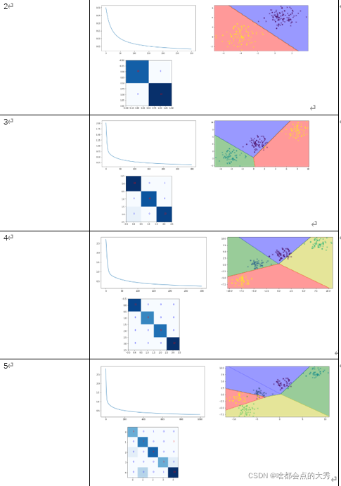
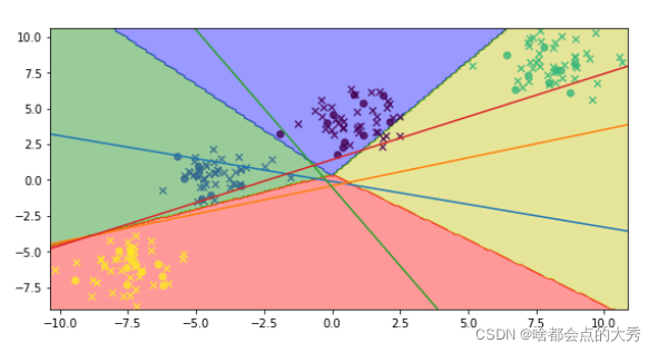
可以看到模型的结果很NICE！！最后，有个问题，大佬们有没有人知道决策边界和参数$\theta$对应的超平面 ${\theta }^{T}X=0$ 是否为相等关系。请解释下图：

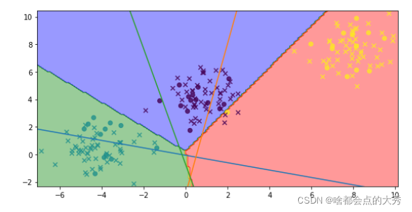
可以看到决策边界和${\theta }^{T}X=0$不是相等关系，下图也是：

---

参考

1.3 种方法实现逻辑回归多分类
2.机器学习：逻辑回归（OvR 与 OvO）
3.逻辑回归 - 4 逻辑回归与多分类
4.一文详解Softmax函数