机器学习-洛杉矶房价预测

老规矩，项目的实际意义，这个也是挺直观的，啰嗦一下买房卖房的时间点很重要哦！！

一、检视原数据集

读入数据并检测

import numpy as np
import pandas as pd
file=open("data/housing/housing.csv")
train_df=pd.read_csv(file)
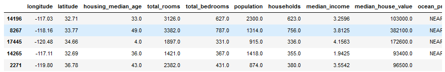
train_df.head()

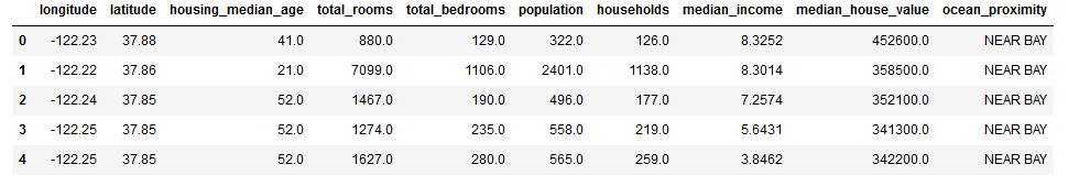上来就给个head()看看数据的样子！！

每一行都表示一个街区。共有 10 个属性：经度、维度、房屋年龄中位数、总房间数、卧室数量、人口数、家庭数、收入中位数、房屋价值中位数、离大海距离。
标准第二个函数

train_df.info()

Output

<class 'pandas.core.frame.DataFrame'>
RangeIndex: 20640 entries, 0 to 20639
Data columns (total 10 columns):
longitude             20640 non-null float64
latitude              20640 non-null float64
housing_median_age    20640 non-null float64
total_rooms           20640 non-null float64
total_bedrooms        20433 non-null float64
population            20640 non-null float64
households            20640 non-null float64
median_income         20640 non-null float64
median_house_value    20640 non-null float64
ocean_proximity       20640 non-null object
dtypes: float64(9), object(1)
memory usage: 1.6+ MB

可以看出total_bedrooms这一项有缺失值，后面要进行处理。ocean_proximity这一项的数据类型为类别型数据
查看具体字段的值的情况

train_df.ocean_proximity.value_counts()

Output

<1H OCEAN     9136
INLAND        6551
NEAR OCEAN    2658
NEAR BAY      2290
ISLAND           5
Name: ocean_proximity, dtype: int64

value_counts()方法查看都有什么类型，每个类都有多少街区
典型操作describe()

train_df.describe()

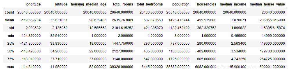这些值很熟悉了吧！！std很重要方差！！

画出每个数值属性的柱状图

%matplotlib inline
from matplotlib import pyplot as plt
plt.style.use('ggplot')
train_df.hist(bins=50,figsize=(16,9))

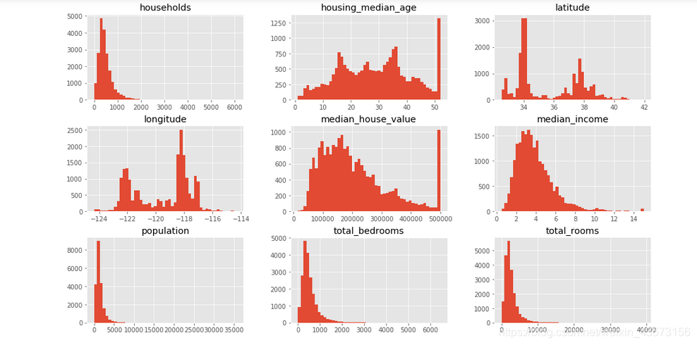
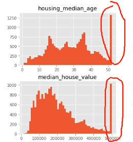
看看上面的图为什么后面的特高呢？就是它把50岁后面的数字全部归到50岁了，设置了一个上限！
同时很多图都可以类似的正态分布来做！！这也是我们想的。
从柱状图中可以发现以下问题：
  1.这些属性的量度不一样，在后面需要进行特征缩放
  2.许多柱状图的尾巴过长，对某些机器学习的算法检测规律会变得更难，所以在后面要处理成正态分布。
  3.房屋年龄中位数和房屋价值中位数也被设了上限。后者可能是个严重的问题，因为它是你的目标属性（你的标签）。你的机器学习算法可能学习到价格不会超出这个界限。你需要与下游团队核实，这是否会成为问题。如果他们告诉你他们需要明确的预测值，即使超过 500000，你则有两个选项：1）对于设了上限的标签，重新收集合适的标签；2）将这些街区从训练集移除（也从测试集移除，因为若房价超出 500000，你的系统就会被差评）。
  4.收入数据经过了缩放处理。
上面的就是你分析数据得到的信息，下面就是如何决策了。

二、创建测试集

目的：防止数据透视偏差。如果一开始就看过测试集，就会不经意间按照其中的规律选择合适的算法，当再用测试集进行评估时，就会导致结果比较乐观，而实际部署时就比较差了。

from sklearn.model_selection import train_test_split # 留出法
train_set,test_set=train_test_split(train_df,test_size=0.2,random_state=42)

train_test_split函数用于将矩阵随机划分为训练子集和测试子集，并返回划分好的训练集测试集样本和训练集测试集标签。 test_size：如果是浮点数，在0-1之间，表示样本占比；如果是整数的话就是样本的数量。random_state：是随机数的种子。产生总是相同的洗牌指数；如果没有这个每次运行会产生不同的测试集，多次之后会得到整个数据集。

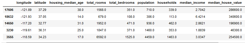
train_set.head(5)#看看数据的情况

不足之处：目前都是采用的纯随机抽样，如果数据量比较小，可能会产生偏差。所以需要关注比较重要的属性，对其进行分层抽样，比如说收入中位数。从直方图中可以看出，大多数的值在2-5（万美元），进行分层抽样时保证每一层都要有足够多的数据，这就意味着，层数不能过多。后面的代码将收入中位数除以1.5（以限制分类的数量），创建收入类别属性，用ceil对值舍入（产生离散的分类），并将大于5的分类归入到分类5。inplace=True原数组内容被改变。
下面代码的意思就是把数据缩放到1-5之间

train_df["income_cat"]=np.ceil(train_df.median_income/1.5)
train_df["income_cat"].where(train_df["income_cat"]<5,5.0,inplace=True)
train_df["income_cat"].head(5)
train_df["income_cat"].value_counts()/len(train_df)

3.0    0.350581
2.0    0.318847
4.0    0.176308
5.0    0.114438
1.0    0.039826
Name: income_cat, dtype: float64

from sklearn.model_selection import StratifiedShuffleSplit # 模型进行分割，进行洗牌操作
split=StratifiedShuffleSplit(n_splits=1,test_size=0.2,random_state=42) # 数据进行洗牌
for train_index,test_index in split.split(train_df,train_df["income_cat"]):
    start_train_set=train_df.loc[train_index]
    start_test_set=train_df.loc[test_index]
start_train_set.head(5)

for set in(start_train_set,start_test_set):
    set.drop(["income_cat"],axis=1,inplace=True)
start_test_set.head(5)

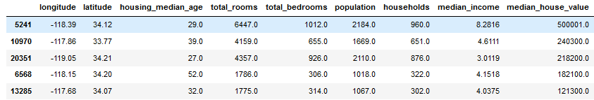需要删除income_cat属性，使数据回到初始状态。

三、数据探索及可视化

目的：以上只是粗略的查看了统计信息，还需要从样本中发现更多的信息。如果训练集非常大，可能还需要采样一个探索集。如果比较小，可以建立一个副本。

housing=start_train_set.copy()

3.1地理数据可视化

原因：样本中有经度和纬度，所以考虑创建散点图

housing.plot(kind="scatter",x="longitude",y="latitude",alpha=0.4,figsize=(15, 10)) # x设置为精度，y设置成纬度， alpha 样本点的透明度
# 样本点颜色重，证明街区多，颜色浅，街区少

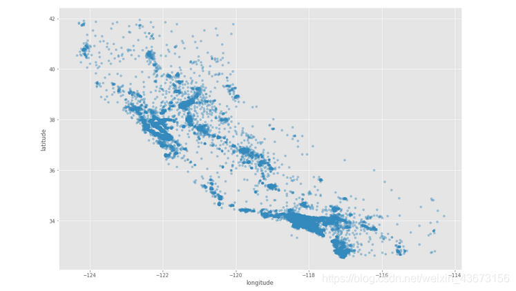
高密度区域：湾区、洛杉矶和圣迭戈等

# s 指 样本点的大小，人口多，散点就达，人口少，样本点小
# c 颜色 越红，证明房价越高

housing.plot(kind="scatter",x="longitude",y="latitude",alpha=0.5,s=housing.population/50,label="population",c=housing.median_house_value,cmap=plt.get_cmap('jet'),colorbar=True,figsize=(15, 10))
plt.legend()

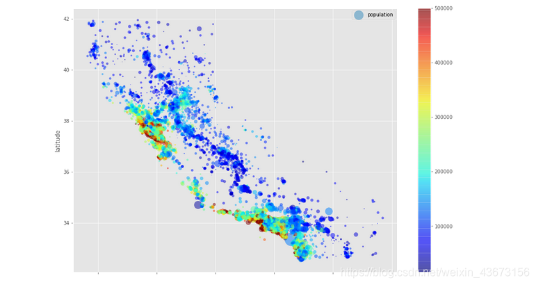
加入人口信息，用点的大小来展示（s）。加入房价信息，用颜色的深浅来表示（c），用预先定义的颜色图“jet”，范围从蓝色到红色，即低价到高价。从图中可以发现房价和位置（沿海地区）以及人口密度存在联系。

import seaborn as sns # matplotlib一个封装
sns.set(style = "whitegrid")#设置样式
x = housing.longitude#X轴数据
y = housing.latitude#Y轴数据
z = housing.median_income#用来调整各个点的大小s
cm = plt.get_cmap('jet')
fig,ax = plt.subplots(figsize = (15,10))
#注意s离散化的方法，因为需要通过点的大小来直观感受其所表示的数值大小
#参数是X轴数据、Y轴数据、各个点的大小、各个点的颜色
bubble = ax.scatter(x, y , s = housing.population/50, c = z, cmap = cm, linewidth = 0.5, alpha = 0.5)
ax.grid()
fig.colorbar(bubble)
ax.set_xlabel('longitude', fontsize = 15)#X轴标签
ax.set_ylabel('latitude', fontsize = 15)#Y轴标签
plt.show()

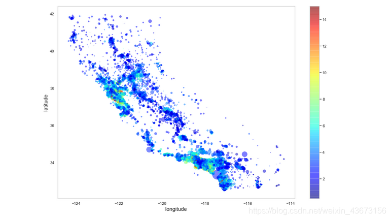
利用seaborn作图也可以达到同样效果。加入人口信息，用点的大小来展示（s）。加入收入信息，用颜色的深浅来表示（c），用预先定义的颜色图“jet”，范围从蓝色到红色，即低价到高价。从图中可以发现收入和位置（沿海地区）以及人口密度存在一定的联系，但是效果不是十分明显。

3.2查看特征之间相关性

corr_matrix=housing.corr()# 统计列与列之间的相关系数
corr_matrix["median_house_value"].sort_values(ascending=False)

Output

median_house_value    1.000000
median_income         0.687160
total_rooms           0.135097
housing_median_age    0.114110
households            0.064506
total_bedrooms        0.047689
population           -0.026920
longitude            -0.047432
latitude             -0.142724
Name: median_house_value, dtype: float64

用热力图的方式展现相关性。annot(annotate的缩写):默认取值False；如果是True，在热力图每个方格写入数据；vmax,vmin:分别是热力图的颜色取值最大和最小范围，默认是根据data数据表里的取值确定。

import seaborn as sns

fig=plt.figure(figsize=(12,8),dpi=80)

sns.heatmap(housing.corr(),annot =True,vmin = 0, vmax = 1)

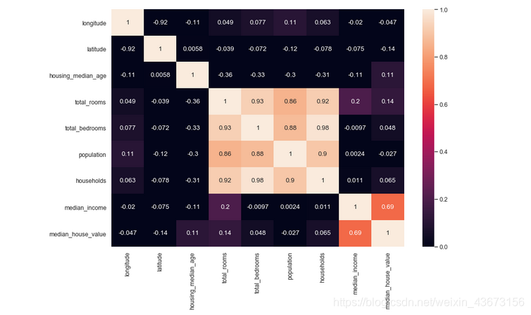
用可视化的方式展现相关性，因为属性过多，所以选取部分属性。

from pandas.plotting import scatter_matrix # 使用散点图矩阵图，可以两两发现特征之间的联系
attributes=["median_house_value","median_income","total_rooms","housing_median_age" ]
scatter_matrix(housing[attributes],figsize=(12,8))

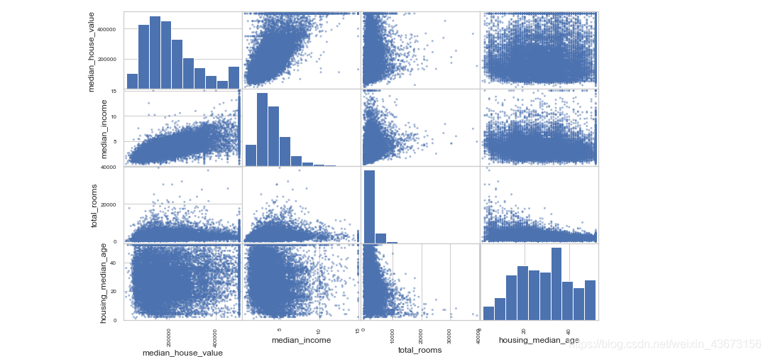
对角线表示每个属性的柱状图。图中可以看出收入对房价的影响还是比较大的，所以可以放大进行研究。

housing.plot(kind="scatter",x="median_income",y="median_house_value",alpha=0.5,figsize=(12,8))

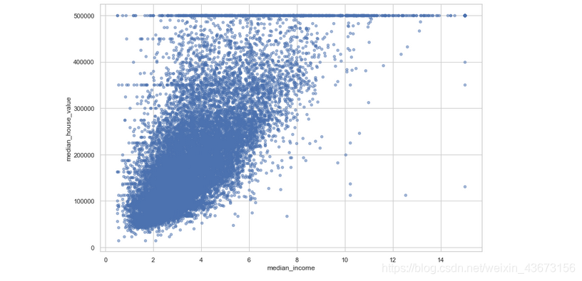
可以看出相关性还是很高的。其次，可以看到一些直线：500000,450000,350000,280000美元，可能是收集资料时设立的边界。

3.3属性组合试验

有一些属性，比如总房间数，在不知道街区有多少户的情况下用处不大。同理总卧室数和总人口数。

housing["rooms_per_household"]=housing.total_rooms/housing.households

housing["bedrooms_per_room"]=housing.total_bedrooms/housing.total_rooms

housing["population_per_household"]=housing.population/housing.households

corr_matrix =housing.corr()

corr_matrix["median_house_value"].sort_values(ascending=False)

Output

median_house_value          1.000000
median_income               0.687160
rooms_per_household         0.146285
total_rooms                 0.135097
housing_median_age          0.114110
households                  0.064506
total_bedrooms              0.047689
population_per_household   -0.021985
population                 -0.026920
longitude                  -0.047432
latitude                   -0.142724
bedrooms_per_room          -0.259984
Name: median_house_value, dtype: float64

间数和卧室数更有信息。而且每户的房间数越多，意味着房屋更大，房价越高，比单纯的看总房间数更有信息

四、数据预处理

目的：为机器学习算法准备数据。
将训练集中预测量和标签分开，因为之后对其要进行不同的转换；drop（）创建备份，不影响原数据集。

# 数据拷贝

housing=start_train_set.drop("median_house_value",axis=1)
housing_copy=housing.copy()
housing_labels=start_train_set.median_house_value.copy()
print(housing.head(5))
print(housing_labels.head(5))

Output

       longitude  latitude  housing_median_age  total_rooms  total_bedrooms  \
17606    -121.89     37.29                38.0       1568.0           351.0   
18632    -121.93     37.05                14.0        679.0           108.0   
14650    -117.20     32.77                31.0       1952.0           471.0   
3230     -119.61     36.31                25.0       1847.0           371.0   
3555     -118.59     34.23                17.0       6592.0          1525.0   

       population  households  median_income ocean_proximity  
17606       710.0       339.0         2.7042       <1H OCEAN  
18632       306.0       113.0         6.4214       <1H OCEAN  
14650       936.0       462.0         2.8621      NEAR OCEAN  
3230       1460.0       353.0         1.8839          INLAND  
3555       4459.0      1463.0         3.0347       <1H OCEAN  
17606    286600.0
18632    340600.0
14650    196900.0
3230      46300.0
3555     254500.0
Name: median_house_value, dtype: float64

4.1数据清洗

目的：处理缺省值。因为很多机器学习算法对缺省值比较敏感（例如LR和SVM，决策树和朴素贝叶斯相对好一点） 思路：
1）去掉缺失的行数据dropna（）；
2）去掉缺失的列drop（）；3）进行赋值fillna（）,可以是0、平均数和中位数。

# 中值填充
median=housing.total_bedrooms.median()
housing.total_bedrooms=housing.total_bedrooms.fillna(median)
housing.isnull().sum().sum()

0

4.2处理文本和类别属性

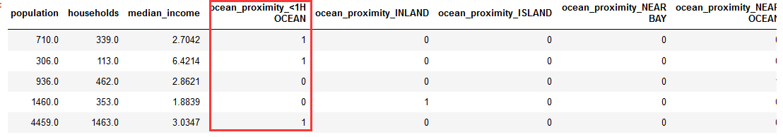
pandas自带的get_dummies方法，可以帮你一键做到One-Hot。
可以看出类别属性ocean_proximity被我们分成了5个column，每一个代表一个category。是就是1，不是就是0。

housing=pd.get_dummies(housing)# onehot

housing.head(5)

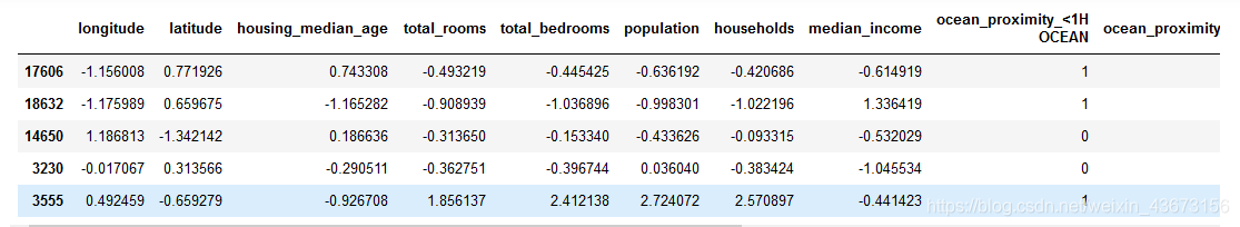
4.3特征缩放

当输入的属性量度不同时，会影响机器学习算法的性能。比如总房间数分布范围在6-39320，收入中位数在0-15。两种方法：归一化和标准化。归一化将数值缩放到0-1之间，标准化不会限定到某个范围，对一些算法有影响，像神经网络算法输入值就必须是0-1。但是异常值对标准化的影响较小。

numeric_cols=housing_copy.columns[housing_copy.dtypes!="object"]

print(numeric_cols)

Output

Index(['longitude', 'latitude', 'housing_median_age', 'total_rooms',
       'total_bedrooms', 'population', 'households', 'median_income'],
      dtype='object')

numeric_col_means = housing.loc[:, numeric_cols].mean()

numeric_col_std = housing.loc[:, numeric_cols].std()

housing.loc[:, numeric_cols] = (housing.loc[:, numeric_cols] - numeric_col_means) /numeric_col_std

housing.head()

housing_labels=(housing_labels-housing_labels.mean())/housing_labels.std() # 标准化处理
housing_labels.head()

17606    0.688047
18632    1.154759
14650   -0.087214
3230    -1.388822
3555     0.410612
Name: median_house_value, dtype: float64

五、模型选择和训练

5.1 在训练集上训练和评估

from sklearn.linear_model import LinearRegression
lin_reg=LinearRegression()

将pandas类型转换为ndarray

X_train=housing.values
X_test=housing_labels.values
print(X_train)
print(X_test)

Output

[[-1.1560078   0.77192624  0.74330838 ...  0.          0.
   0.        ]
 [-1.17598922  0.65967482 -1.16528192 ...  0.          0.
   0.        ]
 [ 1.18681309 -1.34214221  0.18663621 ...  0.          0.
   1.        ]
 ...
 [ 1.58644139 -0.72475939 -1.56290489 ...  0.          0.
   0.        ]
 [ 0.78218944 -0.85104224  0.18663621 ...  0.          0.
   0.        ]
 [-1.43574761  0.99642908  1.85665272 ...  0.          1.
   0.        ]]
[ 0.68804672  1.15475884 -0.08721398 ... -0.94371716  0.16342771
  2.53243254]

先训练一个线性回归模型

lin_reg.fit(X_train,X_test)

Output

LinearRegression(copy_X=True, fit_intercept=True, n_jobs=None,
         normalize=False)

训练完成，用交叉验证法进行模型评估。交叉验证的基本思想是将训练数据集分为k份，每次用k-1份训练模型，用剩余的1份作为验证集。按顺序训练k次后，计算k次的平均误差来评价模型（改变参数后即为另一个模型）的好坏。

from sklearn.model_selection import cross_val_score 
lin_reg_scores=cross_val_score(lin_reg,X_train,X_test,scoring="neg_mean_squared_error",cv=10)
lin_reg_rmse_scores=np.sqrt(-lin_reg_scores)
print(lin_reg_rmse_scores.mean()) # rmse

结果有点糟糕

0.5982833381401739

均方根误差（RMSE），回归任务可靠的性能指标。
利用决策树模型试试看

from sklearn.tree import DecisionTreeRegressor
tree_reg=DecisionTreeRegressor()
tree_reg.fit(X_train,X_test)
tree_reg_scores=cross_val_score(tree_reg,X_train,X_test,scoring="neg_mean_squared_error",cv=10)
tree_reg_rmse_scores=np.sqrt(-tree_reg_scores)
print(tree_reg_rmse_scores.mean())

Output

0.6031006090656957

更糟糕
可以看出决策树模型的误差大于线性回归，性能更差一点。现在选择用随机森林尝试一下。

from sklearn.ensemble import RandomForestRegressor

RF_reg=RandomForestRegressor()

RF_reg.fit(X_train,X_test)

RF_reg_scores=cross_val_score(RF_reg,X_train,X_test,scoring="neg_mean_squared_error",cv=10)
RF_reg_rmse_scores=np.sqrt(-RF_reg_scores)
print(RF_reg_rmse_scores.mean())

0.45254187824239905

随机森林速度慢一点，误差更小，明显更有希望。

5.2 利用网格搜索对模型进行微调

只要提供超参数和试验的值，网格搜索就可以使用交叉验证试验所有可能超参数值的组合。

from sklearn.model_selection import GridSearchCV

param_grid = [

{'n_estimators': [3, 10, 30], 'max_features': [2, 4, 6, 8]},

{'bootstrap': [False], 'n_estimators': [3, 10], 'max_features': [2, 3, 4]},

]

forest_reg = RandomForestRegressor()

grid_search = GridSearchCV(forest_reg, param_grid, cv=5,

scoring='neg_mean_squared_error')

grid_search.fit(X_train,X_test)

Output

GridSearchCV(cv=5, error_score='raise-deprecating',
       estimator=RandomForestRegressor(bootstrap=True, criterion='mse', max_depth=None,
           max_features='auto', max_leaf_nodes=None,
           min_impurity_decrease=0.0, min_impurity_split=None,
           min_samples_leaf=1, min_samples_split=2,
           min_weight_fraction_leaf=0.0, n_estimators='warn', n_jobs=None,
           oob_score=False, random_state=None, verbose=0, warm_start=False),
       fit_params=None, iid='warn', n_jobs=None,
       param_grid=[{'n_estimators': [3, 10, 30], 'max_features': [2, 4, 6, 8]}, {'bootstrap': [False], 'n_estimators': [3, 10], 'max_features': [2, 3, 4]}],
       pre_dispatch='2*n_jobs', refit=True, return_train_score='warn',
       scoring='neg_mean_squared_error', verbose=0)

首先调第一行的参数为n_estimators和max_features，即有34=12种组合，然后再调第二行的参数，即23=6种组合，具体参数的代表的意思以后再讲述。总共组合数为12+6=18种组合。每种交叉验证5次，即18*5=90次模型计算，虽然运算量比较大，但运行完后能得到较好的参数

grid_search.best_params_

Output

{'max_features': 6, 'n_estimators': 30}

可以看到最好参数中30是选定参数的边缘，所以可以再选更大的数试验，可能会得到更好的模型，还可以在8附近选定参数，也可能会得到更好的模型。

grid_search.best_estimator_

Output

RandomForestRegressor(bootstrap=True, criterion='mse', max_depth=None,
           max_features=6, max_leaf_nodes=None, min_impurity_decrease=0.0,
           min_impurity_split=None, min_samples_leaf=1,
           min_samples_split=2, min_weight_fraction_leaf=0.0,
           n_estimators=30, n_jobs=None, oob_score=False,
           random_state=None, verbose=0, warm_start=False)

5.3 用测试集去评估系统

from sklearn.metrics import mean_squared_error
final_model = grid_search.best_estimator_
X_test = start_test_set.drop("median_house_value", axis=1)
y_test = start_test_set["median_house_value"].copy()
median=X_test.total_bedrooms.median()
X_test.total_bedrooms=X_test.total_bedrooms.fillna(median)
X_test=pd.get_dummies(X_test)
numeric_col_means = X_test.loc[:, numeric_cols].mean()
numeric_col_std = X_test.loc[:, numeric_cols].std()
X_test.loc[:, numeric_cols] = (X_test.loc[:, numeric_cols] - numeric_col_means) /numeric_col_std
y_test=(y_test-y_test.mean())/y_test.std()

final_predictions = final_model.predict(X_test)

final_mse = mean_squared_error(y_test, final_predictions)

final_rmse = np.sqrt(final_mse) 

print(final_rmse)

误差

0.4584388288700149

把测试集进行预处理，导入到系统中，误差为0.4584388288700149，模型的表现还不错，没有出现过拟合。

建议： 并没有打印分数 R2的值，误差越小越好，但是对于一个实际案例来说，程度得使用者来定！！！

代码

链接：https://pan.baidu.com/s/1gwFUwmmk0NuShXm5PdoSzQ 
提取码：q6r7