版权声明:本文为博主原创文章,未经博主允许不得转载。 https://blog.csdn.net/dingming001/article/details/81417075
运行环境:win10 64位 py 2.7 pycharm 2018.1.1#!/usr/bin/python
# -*- coding:utf-8 -*-
import numpy as np
import pandas as pd
import matplotlib.pyplot as plt
#导入房价数据
train_df = pd.read_csv('D:/MLCode/SalePrice/input/train.csv', index_col=0)
test_df = pd.read_csv('D:/MLCode/SalePrice/input/test.csv', index_col=0)
#查看前几行
print train_df.head()
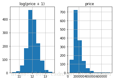
import matplotlib
prices = pd.DataFrame({"price":train_df["SalePrice"], "log(price + 1)":np.log1p(train_df["SalePrice"])})
prices.hist()
plt.show()
#删除saleprice行,合并train,test数据
y_train = np.log1p(train_df.pop('SalePrice'))
all_df = pd.concat((train_df, test_df), axis=0)
y_train.head()
#将数值转化成类型
all_df['MSSubClass'].dtypes
all_df['MSSubClass'] = all_df['MSSubClass'].astype(str)
all_df['MSSubClass'].value_counts()
#进行one-hot编码
pd.get_dummies(all_df['MSSubClass'], prefix='MSSubClass').head()
#我们把所有的category数据,都给One-Hot了
all_dummy_df = pd.get_dummies(all_df)
all_dummy_df.head()
#查看每一列的缺失
all_dummy_df.isnull().sum().sort_values(ascending=False).head(10)
#我们用平均值来填满这些空缺。
mean_cols = all_dummy_df.mean()
mean_cols.head(10)
all_dummy_df = all_dummy_df.fillna(mean_cols)
#看看是不是没有空缺了
all_dummy_df.isnull().sum().sum()
#标准化numerical数据,找到哪些是numerical的列数
numeric_cols = all_df.columns[all_df.dtypes != 'object']
numeric_cols
#归一化处理
numeric_col_means = all_dummy_df.loc[:, numeric_cols].mean()
numeric_col_std = all_dummy_df.loc[:, numeric_cols].std()
all_dummy_df.loc[:, numeric_cols] = (all_dummy_df.loc[:, numeric_cols] - numeric_col_means) / numeric_col_std
#把数据集分回 训练/测试集
dummy_train_df = all_dummy_df.loc[train_df.index]
dummy_test_df = all_dummy_df.loc[test_df.index]
dummy_train_df.shape, dummy_test_df.shape
X_train = dummy_train_df.values
X_test = dummy_test_df.values
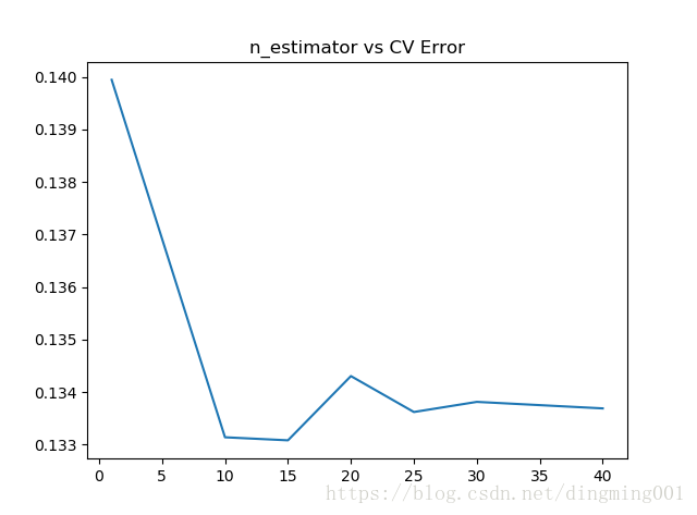
from sklearn.linear_model import Ridge
ridge = Ridge(15)
from sklearn.ensemble import BaggingRegressor
from sklearn.model_selection import cross_val_score
params = [1, 10, 15, 20, 25, 30, 40]
test_scores = []
for param in params:
clf = BaggingRegressor(n_estimators=param, base_estimator=ridge)
test_score = np.sqrt(-cross_val_score(clf, X_train, y_train, cv=10, scoring='neg_mean_squared_error'))
test_scores.append(np.mean(test_score))
import matplotlib.pyplot as plt
plt.plot(params, test_scores)
plt.title("n_estimator vs CV Error")
plt.show()
#Bagging自带的DecisionTree模型
params = [10, 15, 20, 25, 30, 40, 50, 60, 70, 100]
test_scores = []
for param in params:
    clf = BaggingRegressor(n_estimators=param)
    test_score = np.sqrt(-cross_val_score(clf, X_train, y_train, cv=10, scoring='neg_mean_squared_error'))
    test_scores.append(np.mean(test_score))
import matplotlib.pyplot as plt
plt.plot(params, test_scores)
plt.title("n_estimator vs CV Error")
plt.show()
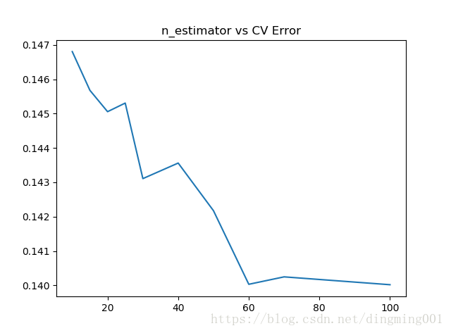
#最好的结果也就0.140
#采用Boosting,Boosting比Bagging理论上更高级点
from sklearn.ensemble import AdaBoostRegressor
params = [10, 15, 20, 25, 30, 35, 40, 45, 50]
test_scores = []
for param in params:
    clf = AdaBoostRegressor(n_estimators=param, base_estimator=ridge)
    test_score = np.sqrt(-cross_val_score(clf, X_train, y_train, cv=10, scoring='neg_mean_squared_error'))
    test_scores.append(np.mean(test_score))
plt.plot(params, test_scores)
plt.title("n_estimator vs CV Error")
plt.show()
#也可以不必输入Base_estimator,使用Adaboost自带的DT
params = [10, 15, 20, 25, 30, 35, 40, 45, 50]
test_scores = []
for param in params:
clf = BaggingRegressor(n_estimators=param)
test_score = np.sqrt(-cross_val_score(clf, X_train, y_train, cv=10, scoring='neg_mean_squared_error'))
test_scores.append(np.mean(test_score))
plt.plot(params, test_scores)
plt.title("n_estimator vs CV Error")
#最后,我们来看看巨牛逼的XGBoost
from xgboost import XGBRegressor
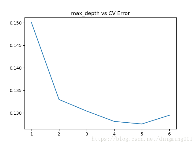
params = [1,2,3,4,5,6]
test_scores = []
for param in params:
clf = XGBRegressor(max_depth=param)
test_score = np.sqrt(-cross_val_score(clf, X_train, y_train, cv=10, scoring='neg_mean_squared_error'))
test_scores.append(np.mean(test_score))
import matplotlib.pyplot as plt
plt.plot(params, test_scores)
plt.title("max_depth vs CV Error")
#深度为5的时候,错误率缩小到0.127