机器学习简单房价预测模型

运行环境：win10 64位 py 2.7 pycharm 2018.1.1

#!/usr/bin/python
# -*- coding:utf-8 -*-
import numpy as np
import pandas as pd
train_df = pd.read_csv('D:/MLCode/SalePrice/input/train.csv', index_col=0)
test_df = pd.read_csv('D:/MLCode/SalePrice/input/test.csv', index_col=0)
train_df.head()
#查看前5行的数据

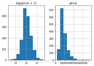
#预测值是偏态，用log转化，最好是正态分布
prices = pd.DataFrame({"price":train_df["SalePrice"], "log(price + 1)":np.log1p(train_df["SalePrice"])})
prices.hist()

这里写图片描述

剩下的部分合并起来
y_train = np.log1p(train_df.pop('SalePrice'))
all_df = pd.concat((train_df, test_df), axis=0)
all_df.shape
#(2919, 79) 去掉y参数之后的行列数，要对其做统一的数据处理

#MSSubClass 的值其实应该是一个category，

#但是Pandas是不会懂这些事儿的。使用DF的时候，这类数字符号会被默认记成数字。

#这种东西就很有误导性，我们需要把它变回成string
all_df['MSSubClass'].dtypes
all_df['MSSubClass'] = all_df['MSSubClass'].astype(str)
all_df['MSSubClass'].value_counts()
#把category的变量转变成numerical表达形式
#当我们用numerical来表达categorical的时候，要注意，数字本身有大小的含义，所以#乱用数字会给之后的模型学习带来麻烦。于是我们可以用One-Hot的方法来表达#category。
pd.get_dummies(all_df['MSSubClass'], prefix='MSSubClass').head()

#同理，我们把所有的category数据，都给One-Hot了
all_dummy_df = pd.get_dummies(all_df)
all_dummy_df.head()

#处理好numerical变量，归一化的处理
all_dummy_df.isnull().sum().sort_values(ascending=False).head(10)
mean_cols = all_dummy_df.mean()
mean_cols.head(10)
all_dummy_df = all_dummy_df.fillna(mean_cols)
all_dummy_df.isnull().sum().sum()
numeric_cols = all_df.columns[all_df.dtypes != 'object']
numeric_cols
numeric_col_means = all_dummy_df.loc[:, numeric_cols].mean()
numeric_col_std = all_dummy_df.loc[:, numeric_cols].std()
all_dummy_df.loc[:, numeric_cols] = (all_dummy_df.loc[:, numeric_cols] - numeric_col_means) / numeric_col_std

处理好数据之后，建立模型
dummy_train_df = all_dummy_df.loc[train_df.index]
dummy_test_df = all_dummy_df.loc[test_df.index]
dummy_train_df.shape, dummy_test_df.shape
#((1460, 303), (1459, 303))
#一个是train数据（不包括price）,一个是test数据

from sklearn.linear_model import Ridge
from sklearn.model_selection import cross_val_score
#只是把DF转化成Numpy Array，这跟Sklearn更加配
X_train = dummy_train_df.values
X_test = dummy_test_df.values

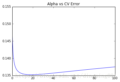
#用Sklearn自带的cross validation方法来测试模型
alphas = np.logspace(-3, 2, 50)
test_scores = []
for alpha in alphas:
    clf = Ridge(alpha)
    test_score = np.sqrt(-cross_val_score(clf, X_train, y_train, cv=10, scoring='neg_mean_squared_error'))
    test_scores.append(np.mean(test_score))

import matplotlib.pyplot as plt
%matplotlib inline
plt.plot(alphas, test_scores)
plt.title("Alpha vs CV Error");

这里写图片描述

#Random Forest，换个模型
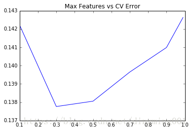
from sklearn.ensemble import RandomForestRegressor
max_features = [.1, .3, .5, .7, .9, .99]
test_scores = []
for max_feat in max_features:
    clf = RandomForestRegressor(n_estimators=200, max_features=max_feat)
    test_score = np.sqrt(-cross_val_score(clf, X_train, y_train, cv=5, scoring='neg_mean_squared_error'))
    test_scores.append(np.mean(test_score))

plt.plot(max_features, test_scores)
plt.title("Max Features vs CV Error");

这里写图片描述

#这里我们用一个Stacking的思维来汲取两种或者多种模型的优点
ridge = Ridge(alpha=15)
rf = RandomForestRegressor(n_estimators=500, max_features=.3)
ridge.fit(X_train, y_train)
rf.fit(X_train, y_train)

#因为最前面我们给label做了个log(1+x), 于是这里我们需要把predit的值给exp回去，#并且减掉那个"1"，所以就是我们的expm1()函数
y_ridge = np.expm1(ridge.predict(X_test))
y_rf = np.expm1(rf.predict(X_test))

y_ridge = np.expm1(ridge.predict(X_test))
y_rf = np.expm1(rf.predict(X_test))

#做个简单的优化
y_final = (y_ridge + y_rf) / 2

submission_df = pd.DataFrame(data= {'Id' : test_df.index, 'SalePrice': y_final})

得到了一个简单的结果

机器学习简单房价预测模型

猜你喜欢