文章目录

1. PCA介绍
- 1.1 概念
- 1.2 降维及恢复示意图
2. PCA 算法模拟
- 2.1 Numpy实现
- 2.2 sklearn 包实现
3. 实例：pca进行人脸降维

%matplotlib inline
import matplotlib.pyplot as plt
import numpy as np

1. PCA介绍

1.1 概念

思想：
在这里插入图片描述

dots = np.array([[1, 1.5], [2, 1.5], [3, 3.6], [4, 3.2], [5, 5.5]])

def cross_point(x0, y0):
    """
    1. line1: y = x
    2. line2: y = -x + b => x = b/2
    3. [x0, y0] is in line2 => b = x0 + y0

    => x1 = b/2 = (x0 + y0) / 2
    => y1 = x1
    """
    x1 = (x0 + y0) / 2
    return x1, x1


plt.figure(figsize=(8, 6), dpi=144)
plt.title('2-dimension to 1-dimension')

plt.xlim(0, 8)
plt.ylim(0, 6)
ax = plt.gca()                                  # gca 代表当前坐标轴，即 'get current axis'
ax.spines['right'].set_color('none')            # 隐藏坐标轴
ax.spines['top'].set_color('none')

plt.scatter(dots[:, 0], dots[:, 1], marker='s', c='b')
plt.plot([0.5, 6], [0.5, 6], '-r')
for d in dots:
    x1, y1 = cross_point(d[0], d[1])
    plt.plot([d[0], x1], [d[1], y1], '--b')
    plt.scatter(x1, y1, marker='o', c='r')
plt.annotate(r'projection point',
             xy=(x1, y1), xycoords='data',
             xytext=(x1 + 0.5, y1 - 0.5), fontsize=10,
             arrowprops=dict(arrowstyle="->", connectionstyle="arc3,rad=.2"))
plt.annotate(r'vector $u^{(1)}$',
             xy=(4.5, 4.5), xycoords='data',
             xytext=(5, 4), fontsize=10,
             arrowprops=dict(arrowstyle="->", connectionstyle="arc3,rad=.2"))

[外链图片转存失败,源站可能有防盗链机制,建议将图片保存下来直接上传(img-D5EdefSF-1631534761083)(output_1_18.png)]
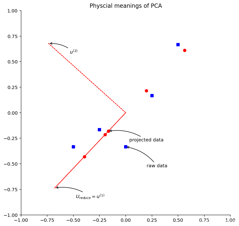
图中正方形的点是原始数据经过预处理后（归一化、缩放）的数据，圆形的点是从一维恢复到二维后的数据。同时，我们画出主成分特征向量u1,u2 。根据上图，来介绍几个有意思的结论：首先，圆形的点实际上就是方形的点在向量u1,u2 所在直线上的投影。所谓PCA数据恢复，并不是真正的恢复，只是把降维后的坐标转换为原坐标系中的坐标而已。针对我们的例子，只是把由向量u1,u2 决定的一维坐标系中的坐标转换为原始二维坐标系中的坐标。其次，主成分特征向量u1,u2是相互垂直的。再次，方形点和圆形点之间的距离，就是PCA数据降维后的误差。

1.2 降维及恢复示意图

plt.figure(figsize=(8, 8), dpi=144)

plt.title('Physcial meanings of PCA')

ymin = xmin = -1
ymax = xmax = 1
plt.xlim(xmin, xmax)
plt.ylim(ymin, ymax)
ax = plt.gca()                                  # gca 代表当前坐标轴，即 'get current axis'
ax.spines['right'].set_color('none')            # 隐藏坐标轴
ax.spines['top'].set_color('none')

plt.scatter(norm[:, 0], norm[:, 1], marker='s', c='b')
plt.scatter(Z[:, 0], Z[:, 1], marker='o', c='r')
plt.arrow(0, 0, U[0][0], U[1][0], color='r', linestyle='-')
plt.arrow(0, 0, U[0][1], U[1][1], color='r', linestyle='--')
plt.annotate(r'$U_{reduce} = u^{(1)}$',
             xy=(U[0][0], U[1][0]), xycoords='data',
             xytext=(U_reduce[0][0] + 0.2, U_reduce[1][0] - 0.1), fontsize=10,
             arrowprops=dict(arrowstyle="->", connectionstyle="arc3,rad=.2"))
plt.annotate(r'$u^{(2)}$',
             xy=(U[0][1], U[1][1]), xycoords='data',
             xytext=(U[0][1] + 0.2, U[1][1] - 0.1), fontsize=10,
             arrowprops=dict(arrowstyle="->", connectionstyle="arc3,rad=.2"))
plt.annotate(r'raw data',
             xy=(norm[0][0], norm[0][1]), xycoords='data',
             xytext=(norm[0][0] + 0.2, norm[0][1] - 0.2), fontsize=10,
             arrowprops=dict(arrowstyle="->", connectionstyle="arc3,rad=.2"))
plt.annotate(r'projected data',
             xy=(Z[0][0], Z[0][1]), xycoords='data',
             xytext=(Z[0][0] + 0.2, Z[0][1] - 0.1), fontsize=10,
             arrowprops=dict(arrowstyle="->", connectionstyle="arc3,rad=.2"))

Text(0.03390904029252009, -0.28050757997562326, 'projected data')

在这里插入图片描述

2. PCA 算法模拟

2.1 Numpy实现

A = np.array([[3, 2000], 
              [2, 3000], 
              [4, 5000], 
              [5, 8000], 
              [1, 2000]], dtype='float')

# 数据归一化
mean = np.mean(A, axis=0)
norm = A - mean
# 数据缩放
scope = np.max(norm, axis=0) - np.min(norm, axis=0)
norm = norm / scope
norm

array([[ 0.        , -0.33333333],
       [-0.25      , -0.16666667],
       [ 0.25      ,  0.16666667],
       [ 0.5       ,  0.66666667],
       [-0.5       , -0.33333333]])

U, S, V = np.linalg.svd(np.dot(norm.T, norm))
U

array([[-0.67710949, -0.73588229],
       [-0.73588229,  0.67710949]])

U_reduce = U[:, 0].reshape(2,1)
U_reduce

array([[-0.67710949],
       [-0.73588229]])

R = np.dot(norm, U_reduce)
R

array([[ 0.2452941 ],
       [ 0.29192442],
       [-0.29192442],
       [-0.82914294],
       [ 0.58384884]])

Z = np.dot(R, U_reduce.T)
Z

array([[-0.16609096, -0.18050758],
       [-0.19766479, -0.21482201],
       [ 0.19766479,  0.21482201],
       [ 0.56142055,  0.6101516 ],
       [-0.39532959, -0.42964402]])

np.multiply(Z, scope) + mean

array([[2.33563616e+00, 2.91695452e+03],
       [2.20934082e+00, 2.71106794e+03],
       [3.79065918e+00, 5.28893206e+03],
       [5.24568220e+00, 7.66090960e+03],
       [1.41868164e+00, 1.42213588e+03]])

2.2 sklearn 包实现

from sklearn.decomposition import PCA
from sklearn.pipeline import Pipeline
from sklearn.preprocessing import MinMaxScaler

def std_PCA(**argv):
    # MinMaxScaler对数据进行预处理
    scaler = MinMaxScaler()
    # PCA算法
    pca = PCA(**argv)
    pipeline = Pipeline([('scaler', scaler),
                         ('pca', pca)])
    return pipeline

pca = std_PCA(n_components=1)
R2 = pca.fit_transform(A)
R2

array([[-0.2452941 ],
       [-0.29192442],
       [ 0.29192442],
       [ 0.82914294],
       [-0.58384884]])

pca.inverse_transform(R2)

array([[2.33563616e+00, 2.91695452e+03],
       [2.20934082e+00, 2.71106794e+03],
       [3.79065918e+00, 5.28893206e+03],
       [5.24568220e+00, 7.66090960e+03],
       [1.41868164e+00, 1.42213588e+03]])

3. 实例：pca进行人脸降维

%matplotlib inline
import matplotlib.pyplot as plt
import numpy as np

from sklearn.datasets import fetch_olivetti_faces

# fetch_olivetti_faces函数可以帮助我们截取中间部分，只留下脸部特征
faces = fetch_olivetti_faces(data_home='datasets/')

X = faces.data
y = faces.target
image = faces.images
print("data:{}, label:{}, image:{}".format(X.shape, y.shape, image.shape))

data:(400, 4096), label:(400,), image:(400, 64, 64)

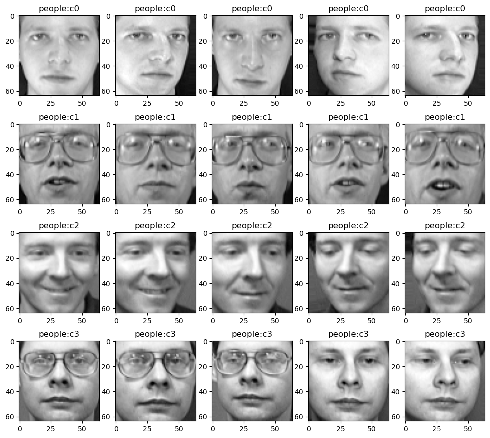
查看部分图像

target_names = np.array(["c%d" % i for i in np.unique(y)])
target_names

array(['c0', 'c1', 'c2', 'c3', 'c4', 'c5', 'c6', 'c7', 'c8', 'c9', 'c10',
       'c11', 'c12', 'c13', 'c14', 'c15', 'c16', 'c17', 'c18', 'c19',
       'c20', 'c21', 'c22', 'c23', 'c24', 'c25', 'c26', 'c27', 'c28',
       'c29', 'c30', 'c31', 'c32', 'c33', 'c34', 'c35', 'c36', 'c37',
       'c38', 'c39'], dtype='<U3')

plt.figure(figsize=(12, 11), dpi=100)

# 这里显示两个人的各5张图像
shownum = 40
# 提取前k个人的名字
title = target_names[:int(shownum/10)]
j = 1

# 每个人的10张图像主题曲前面的5张来展示
for i in range(shownum):
    if i%10 < 5:
        plt.subplot(int(shownum/10),5,j)
        plt.title("people:"+title[int(i/10)])
        plt.imshow(image[i],cmap=plt.cm.gray)
        j+=1

在这里插入图片描述

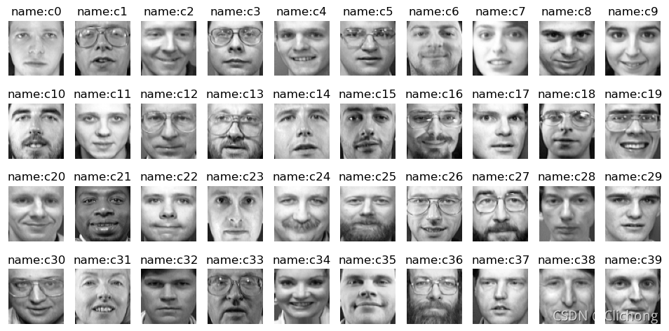
提取全部40人的第一张图像,并进行展示

subimage = None

for i in range(len(image)):
    if i%10 == 0:
        if subimage is not None:
#             print("subimage.shape:{},image[i].shape:{}",subimage.shape, image[i].shape)
            subimage = np.concatenate((subimage, image[i].reshape(1,64,64)), axis=0)
        else:
            subimage = image[i].reshape(1,64,64)
            
plt.figure(figsize=(12,6), dpi=100)

for i in range(subimage.shape[0]):
    plt.subplot(int(subimage.shape[0]/10), 10, i+1)
    plt.imshow(subimage[i], cmap=plt.cm.gray)
    plt.title("name:"+target_names[i])
    plt.axis('off')

在这里插入图片描述
划分数据集

from sklearn.model_selection import train_test_split

X_train, X_test, y_train, y_test = train_test_split(
    X, y, test_size=0.2, random_state=4)

X_train.shape, X_test.shape, y_train.shape, y_test.shape

((320, 4096), (80, 4096), (320,), (80,))

使用svm来实现人脸识别

from sklearn.svm import SVC

# 指定SVC的class_weight参数，让SVC模型能根据训练样本的数量来均衡地调整权重
clf = SVC(class_weight='balanced')
# 训练
clf.fit(X_train, y_train)
# 计算得分
trainscore = clf.score(X_train,y_train)
testscore = clf.score(X_test,y_test)
print("trainscore:{},testscore:{}".format(trainscore, testscore))
# 预测
y_pred = clf.predict(X_test)

trainscore:1.0,testscore:0.975

显示图像测试集图像

# plt.figure(figsize=(12,6), dpi=100)
plt.subplot(1,1,1)
plt.imshow(X_test[1].reshape(64,64), cmap=plt.cm.gray)

<matplotlib.image.AxesImage at 0x21fb6d83688>

在这里插入图片描述

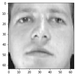
预测是正确的，可以发现svm的预测效果非常好

y_test[1] == y_pred[1]

True

其中PCA模型的explained_variance_ratio变量可以获取经PCA处理后的数据还原率

from sklearn.decomposition import PCA

pca = PCA(n_components=140)
X_pca = pca.fit_transform(X)
np.sum(pca.explained_variance_ratio_)

0.9585573

现在使用的是4096个特征，现在使用PCA对特征进行降维，再查看图像的变化;

from sklearn.decomposition import PCA

# 原图展示
plt.figure(figsize=(12,8), dpi=100)
subimage = faces.images[:5]
for i in range(5):
    plt.subplot(1, 5, i+1)
    plt.imshow(subimage[i], cmap=plt.cm.gray)
    plt.axis('off')
    
# 降维后的图片展示
k = [140, 75, 37, 19, 8]
plt.figure(figsize=(12,12), dpi=100)

for index in range(len(k)):
    pca = PCA(n_components=k[index])

    # 进行降维处理
    X_pca = pca.fit_transform(X)
    # 重新升维，中间过程有损耗
    X_invert_pca = pca.inverse_transform(X_pca)
    image = X_invert_pca.reshape(-1,64,64)
    subimage = image[:5]
    
    for i in range(len(k)):
        plt.subplot(len(k), 5, (i+1)+len(k)*index)
        plt.imshow(subimage[i], cmap=plt.cm.gray)
    #     plt.title("name:"+target_names[i])
        plt.axis('off')

[外链图片转存失败,源站可能有防盗链机制,建议将图片保存下来直接上传(img-OhWWKD17-1631534950314)(output_32_0.png)]

可以看见降维后的人脸逐渐模糊，从4096特征维度讲到140维度还是可以保持脸部的大部分特征

https://zhuanlan.zhihu.com/p/271969151 关于 fit(), transform(), fit_transform()区别，这篇博客有介绍

必须先用fit_transform(trainData)，之后再transform(testData)。如果直接transform(testData)，程序会报错

如果fit_transfrom(trainData)后，使用fit_transform(testData)而不transform(testData)，虽然也能归一化，但是两个结果不是在同一个“标准”下的，具有明显差异。也就是我们需要用处理训练集的归一化过程来处理测试集，确保有相同的数据处理。

from sklearn.svm import SVC

# 设定多降到的维度
pca = PCA(n_components=140)

# 先使用训练集对进行训练与归一化处理
X_train_pca = pca.fit_transform(X_train)
# 然后对测试采用训练集同样的参数进行归一化处理
X_test_pca = pca.transform(X_test)

# 指定SVC的class_weight参数，让SVC模型能根据训练样本的数量来均衡地调整权重
clf = SVC(class_weight='balanced')
# 用归一化后的数据给svm进行训练
clf.fit(X_train_pca, y_train)

# 计算得分
trainscore = clf.score(X_train_pca,y_train)
testscore = clf.score(X_test_pca,y_test)
print("trainscore:{},testscore:{}".format(trainscore, testscore))

trainscore:1.0,testscore:0.975

使用GridSearchCV来进一步筛选

from sklearn.model_selection import GridSearchCV

# print("Searching the best parameters for SVC ...")
param_grid = {
    
    'C': [1, 5, 10, 50, 100],
              'gamma': [0.0001, 0.0005, 0.001, 0.005, 0.01]}
clf = GridSearchCV(SVC(kernel='rbf', class_weight='balanced'), param_grid, verbose=2, n_jobs=4)
clf = clf.fit(X_train_pca, y_train)
print("Best parameters found by grid search:",clf.best_params_)

# 计算得分
trainscore = clf.score(X_train_pca,y_train)
testscore = clf.score(X_test_pca,y_test)
print("trainscore:{},testscore:{}".format(trainscore, testscore))

Fitting 5 folds for each of 25 candidates, totalling 125 fits
Best parameters found by grid search: {'C': 5, 'gamma': 0.005}
trainscore:1.0,testscore:0.9625

可以看见效果还是非常不错的

import pandas as pd

result = pd.DataFrame()
result['pred'] = y_pred
result['true'] = y_test
result['compares'] = y_pred==y_test
result.head(10)

	pred	true	compares
0	18	18	True
1	0	0	True
2	6	6	True
3	31	31	True
4	10	10	True
5	27	27	True
6	36	36	True
7	32	32	True
8	29	29	True
9	33	33	True

机器学习原理与实战 | PCA降维实践

文章目录

1. PCA介绍

1.1 概念

1.2 降维及恢复示意图

2. PCA 算法模拟

2.1 Numpy实现

2.2 sklearn 包实现

3. 实例：pca进行人脸降维

猜你喜欢