Glow: Generative Flow with Invertible 1×1 Convolutions
![]()
目录
Glow: Generative Flow with Invertible 1×1 Convolutions
Background: Flow-based Generative Models
1. Actnorm: scale and bias layer with data dependent initialization
2. Invertible 1 × 1 convolution
Abstract
Flow-based generative models (Dinh et al., 2014) are conceptually attractive due to tractability of the exact log-likelihood, tractability of exact latent-variable inference, and parallelizability of both training and synthesis.
In this paper we propose Glow, a simple type of generative flow using an invertible 1 × 1 convolution. Using our method we demonstrate a significant improvement in log-likelihood on standard benchmarks. Perhaps most strikingly, we demonstrate that a generative model optimized towards the plain log-likelihood objective is capable of efficient realistic-looking synthesis and manipulation of large images.
基于流程的生成模型 (Dinh et al., 2014) 在概念上很有吸引力,因为精确对数似然的可加工性,精确潜在变量推断的可加工性,以及训练和合成的并行性。本文提出 Glow,一个简单类型的生成流使用可逆的 1 × 1卷积。该方法在标准基准上对数似然的显著改进。也许最引人注目的是,我们证明了优化到简单对数似然目标的生成模型能够有效地逼真地合成和处理大图像。
(Dinh et al., 2014) NICE: non-linear independent components estimation [2015 ICLR]
Introduction
Two major unsolved problems in the field of machine learning are (1) data-efficiency: the ability to learn from few datapoints, like humans; and (2) generalization: robustness to changes of the task or its context. AI systems, for example, often do not work at all when given inputs that are different from their training distribution.
A promise of generative models, a major branch of machine learning, is to overcome these limitations by: (1) learning realistic world models, potentially allowing agents to plan in a world model before actual interaction with the world, and (2) learning meaningful features of the input while requiring little or no human supervision or labeling.
Since such features can be learned from large unlabeled datasets and are not necessarily task-specific, downstream solutions based on those features could potentially be more robust and more data efficient.
In this paper we work towards this ultimate vision, in addition to intermediate applications, by aiming to improve upon the state-of-the-art of generative models.
研究动机:本文的研究动机很高级
机器学习领域中两个尚未解决的主要问题是: (1) 数据效率: 像人类一样从少数数据点学习的能力; (2) 泛化: 对任务或其上下文变化的鲁棒性。以人工智能系统为例,如果输入的输入与训练分布不同,它通常根本无法工作。
生成模型、机器学习的一个主要分支,是克服这些限制: (1) 学习真实世界模型,可能允许代理计划在世界模型实际与世界互动,和 (2) 学习输入的有意义特征需要很少或根本没有人监督或标签。
由于这些特性可以从大型未标记的数据集中学习,而且不一定是特定于任务的,因此基于这些特性的下游解决方案可能更鲁棒,数据效率更高。
本文致力于这个最终的愿景,除了中间的应用,旨在改进最先进的生成模型。
Generative modeling is generally concerned with the extremely challenging task of modeling all dependencies within very high-dimensional input data, usually specified in the form of a full joint probability distribution. Since such joint models potentially capture all patterns that are present in the data, the applications of accurate generative models are near endless. Immediate applications are as diverse as speech synthesis, text analysis, semi-supervised learning and model-based control; see Section 4 for references.
生成建模通常涉及到在非常高维的输入数据中建模所有依赖项这一极具挑战性的任务,通常以完整的联合概率分布的形式指定。由于这种联合模型可能捕获数据中存在的所有模式,精确生成模型的应用几乎是无穷无尽的。即时应用包括语音合成、文本分析、半监督学习和基于模型的控制; 参考第 4 节。
The discipline of generative modeling has experienced enormous leaps in capabilities in recent years, mostly with likelihood-based methods (Graves, 2013; Kingma and Welling, 2013, 2018; Dinh et al., 2014; van den Oord et al., 2016a) and generative adversarial networks (GANs) (Goodfellow et al., 2014) (see Section 4). Likelihood-based methods can be divided into three categories:
1. Autoregressive models (Hochreiter and Schmidhuber, 1997; Graves, 2013; van den Oord et al., 2016a,b; Van Den Oord et al., 2016). Those have the advantage of simplicity, but have as disadvantage that synthesis has limited parallelizability, since the computational length of synthesis is proportional to the dimensionality of the data; this is especially troublesome for large images or video.
2. Variational autoencoders (VAEs) (Kingma and Welling, 2013, 2018), which optimize a lower bound on the log-likelihood of the data. Variational autoencoders have the advantage of parallelizability of training and synthesis, but can be comparatively challenging to optimize (Kingma et al., 2016).
3. Flow-based generative models, first described in NICE (Dinh et al., 2014) and extended in RealNVP (Dinh et al., 2016). We explain the key ideas behind this class of model in the following sections.
生成建模的学科在近年来经历了巨大的飞跃,主要是基于似然的方法 (Graves, 2013; Kingma 与Welling,2013,2018; Dinh et al., 2014; van den Oord et al., 2016a) 和生成式对抗网络 (GAN) (Goodfellow et al., 2014) (见第 4 节)。基于似然的方法可分为三类:
1. 自回归模型。这些方法的优点是简单,但缺点是合成的并行性有限,因为合成的计算长度与数据的维数成正比; 这对于大图像或视频来说尤其麻烦。
2. 变分自编码器 (VAEs) ,优化数据对数似然的下界。变分自编码器具有训练和合成并行性的优势,但优化相对具有挑战性 (Kingma et al., 2016)。
3. 基于流的生成模型,首先在 NICE (Dinh et al., 2014)中描述,并在 RealNVP 中扩展 (Dinh et al., 2016)。我们将在下面几节中解释这类模型背后的关键思想。
NICE: Non-linear independent components estimation. [2015 ICLR]
Density estimation using Real NVP. [2017 ICLR]
Flow-based generative models have so far gained little attention in the research community compared to GANs (Goodfellow et al., 2014) and VAEs (Kingma and Welling, 2013). Some of the merits of flow-based generative models include:
• Exact latent-variable inference and log-likelihood evaluation. In VAEs, one is able to infer only approximately the value of the latent variables that correspond to a datapoint. GAN’s have no encoder at all to infer the latents. In reversible generative models, this can be done exactly without approximation. Not only does this lead to accurate inference, it also enables optimization of the exact log-likelihood of the data, instead of a lower bound of it.
• Efficient inference and efficient synthesis. Autoregressive models, such as the PixelCNN (van den Oord et al., 2016b), are also reversible, however synthesis from such models is difficult to parallelize, and typically inefficient on parallel hardware. Flow-based generative models like Glow (and RealNVP) are efficient to parallelize for both inference and synthesis.
• Useful latent space for downstream tasks. The hidden layers of autoregressive models have unknown marginal distributions, making it much more difficult to perform valid manipulation of data. In GANs, datapoints can usually not be directly represented in a latent space, as they have no encoder and might not have full support over the data distribution (Grover et al., 2018). This is not the case for reversible generative models and VAEs, which allow for various applications such as interpolations between datapoints and meaningful modifications of existing datapoints.
• Significant potential for memory savings. Computing gradients in reversible neural networks requires an amount of memory that is constant instead of linear in their depth, as explained in the RevNet paper (Gomez et al., 2017).
与 GANs 和 VAEs 相比,迄今为止,基于流的生成模型在研究界受到的关注很少。基于流程的生成模型的一些优点包括:
• 准确的潜在变量推断和对数似然评估。在 VAEs 中,人们只能推断出与数据点相对应的潜在变量的近似值。GAN 没有任何编码器来推断潜势。在可逆的生成模型中,这可以完全不需要近似。这不仅可以得到准确的推断,还可以优化数据的准确日志可能性,而不是数据的下界。
• 高效的推理和高效的合成。自回归模型,如 PixelCNN (van den Oord et al., 2016b),也是可逆的,但是从这些模型合成很难并行化,并且在并行硬件上通常效率低下。Glow (和 RealNVP) 等基于流的生成模型能够有效地并行化推理和合成。
• 对下游任务有用的潜在空间。自回归模型的隐藏层具有未知的边际分布,使得数据的有效操作更加困难。在 GAN 中,数据点通常不能直接在潜在空间中表示,因为它们没有编码器,而且可能没有对数据分布的完全支持。可逆生成模型和 VAEs 没有这种情况,它们允许各种应用程序,如数据点之间的插值和现有数据点的有意义的修改。
• 节省内存的巨大潜力。正如 RevNet 论文中解释的那样,在可逆神经网络中计算梯度需要的内存数量是恒定的,而不是深度上线性的 (Gomez等人,2017)。
In this paper we propose a new a generative flow coined Glow, with various new elements as described in Section 3. In Section 5, we compare our model quantitatively with previous flows, and in Section 6, we study the qualitative aspects of our model on high-resolution datasets.
在本文中,我们提出了一个新的生成流,即 Glow,在第 3 节中描述的各种新元素。在第 5 节中,该模型与之前的流进行了定量比较,在第 6 节中,定性地研究了该模型在高分辨率数据集上 的表现。
Background: Flow-based Generative Models
Let x be a high-dimensional random vector with unknown true distribution
. We collect an i.i.d. dataset D, and choose a model
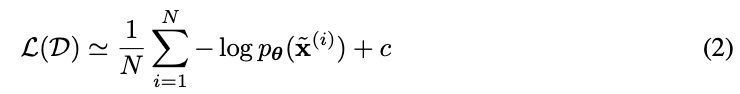
with parameters θ. In case of discrete data x, the log-likelihood objective is then equivalent to minimizing:
In case of continuous data x, we minimize the following:
where
with
, and
where a is determined by the discretization level of the data and M is the dimensionality of x. Both objectives (eqs. (1) and (2)) measure the expected compression cost in nats or bits; see (Dinh et al., 2016). Optimization is done through stochastic gradient descent using minibatches of data (Kingma and Ba, 2015).

设 x 是一个真实分布未知的高维随机向量 。收集一个 i.i.d. 数据集 D,并选择一个参数为 θ 的模型
。对于离散数据 x,则对数似然目标等价于最小化 (1)。对于连续数据 x,最小化如 (2)。其中
with
,
,其中 a 由数据的离散化程度决定,M是x的维数。(1) 和m(2)) 以 nats 或 bits 度量预期的压缩成本; 见 (Dinh et al., 2016)。通过使用小批量数据的随机梯度下降进行优化 (Kingma和Ba, 2015)。
In most flow-based generative models (Dinh et al., 2014, 2016), the generative process is defined as:
where z is the latent variable and pθ(z) has a (typically simple) tractable density, such as a spherical multivariate Gaussian distribution:
. The function gθ(..) is invertible, also called bijective, such that given a datapoint x, latent-variable inference is done by
. For brevity, we will omit subscript θ from fθ and gθ.
在大多数基于流程的生成模型(Dinh et al., 2014, 2016)中,生成过程被定义为 (3) 和 (4)。
其中 z 为潜变量,pθ(z)具有(通常简单的)易于处理的密度,如球形多元高斯分布。gθ(..) 是可逆的,也称为双射,因此给定一个数据点 x,可以通过
进行潜变量推断。为了简便起见,我们将 fθ 和 gθ 中的下标 θ 省略。
We focus on functions where f (and, likewise, g) is composed of a sequence of transformations: f = f1 ◦ f2 ◦ · · · ◦ fK, such that the relationship between x and z can be written as:
我们关注 f (和 g 同样) 由一系列变换组成的函数: f = f1◦f2◦···◦fK,这样 x 和 z 之间的关系可以写成 (5)。
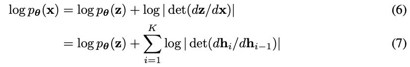
Such a sequence of invertible transformations is also called a (normalizing) flow (Rezende and Mohamed, 2015). Under the change of variables of eq. (4), the probability density function (pdf) of the model given a datapoint can be written as:
where we define
and
for conciseness. The scalar value log | det(dhi/dhi−1)| is the logarithm of the absolute value of the determinant of the Jacobian matrix (dhi/dhi−1), also called the log-determinant. This value is the change in log-density when going from hi−1 to hi under transformation fi . While it may look intimidating, its value can be surprisingly simple to compute for certain choices of transformations, as previously explored in (Deco and Brauer, 1995; Dinh et al., 2014; Rezende and Mohamed, 2015; Kingma et al., 2016). The basic idea is to choose transformations whose Jacobian dhi/dhi−1 is a triangular matrix. For those transformations, the log-determinant is simple:
where sum() takes the sum over all vector elements, log() takes the element-wise logarithm, and diag() takes the diagonal of the Jacobian matrix.
这种可逆变换序列也称为(标准化)流。在式 (4) 变量的变化下,模型给定数据点的概率密度函数(pdf) 可表示为 (6) 和 (7)。
为了简洁,定义 and
。标量值 log | det(dhi/dhi−1)| 为雅可比矩阵行列式绝对值(dhi/dhi−1) 的对数,也称对数行列式。这个值是在变换 fi 下从 hi−1 到 hi 时的对数密度变化。虽然它可能看起来令人生畏,但它的价值可以令人惊讶地简单地计算某些转换的选择。基本思想是选择其雅可比矩阵 dhi/dhi−1 是一个三角矩阵的变换。对于这些变换,对数行列式很简单,如 (8)。其中 sum() 取所有向量元素的和,log() 取元素对数,diag() 取雅可比矩阵的对角线。
Proposed Generative Flow
We propose a new flow, building on the NICE and RealNVP flows proposed in (Dinh et al., 2014, 2016). It consists of a series of steps of flow, combined in a multi-scale architecture; see Figure 2. Each step of flow consists of actnorm (Section 3.1) followed by an invertible 1 × 1 convolution (Section 3.2), followed by a coupling layer (Section 3.3).
This flow is combined with a multi-scale architecture; due to space constraints we refer to (Dinh et al., 2016) for more details. This architecture has a depth of flow K, and number of levels L (Figure 2).
我们提出了一个新的流程,建立在 NICE 和 RealNVP 流的基础上。它由一系列流的步骤组成,结合在一个多尺度的体系结构中; 参见图2。流的每一步包括 actnorm (第3.1节),然后是可逆的 1 × 1卷积 invertible 1 × 1 convolution (第3.2节),然后是耦合层 coupling layer (第3.3节)。
该流程与多尺度架构相结合;由于空间限制,我们参考(Dinh et al., 2016)了解更多细节。该体系结构具有流的深度K,级别的数量L(图2)。

1. Actnorm: scale and bias layer with data dependent initialization
In Dinh et al. (2016), the authors propose the use of batch normalization (Ioffe and Szegedy, 2015) to alleviate the problems encountered when training deep models. However, since the variance of activations noise added by batch normalization is inversely proportional to minibatch size per GPU or other processing unit (PU), performance is known to degrade for small per-PU minibatch size. For large images, due to memory constraints, we learn with minibatch size 1 per PU. We propose an actnorm layer (for activation normalizaton), that performs an affine transformation of the activations using a scale and bias parameter per channel, similar to batch normalization. These parameters are initialized such that the post-actnorm activations per-channel have zero mean and unit variance given an initial minibatch of data. This is a form of data dependent initialization (Salimans and Kingma, 2016). After initialization, the scale and bias are treated as regular trainable parameters that are independent of the data.
在 Dinh 等人 (2016) 中,作者提出使用批归一化来缓解训练深度模型时遇到的问题。然而,由于批处理归一化所增加的激活噪声的方差与每个 GPU 或其他处理单元 (PU) 的 minibatch 大小成反比,性能已知在每个 PU 的 minibatch 大小较小时下降。对于大的图像,由于内存的限制,学习每 PU 的 minibatch 大小为 1。
本文提出一个 actnorm 层 (用于激活归一化),它使用每个通道的尺度和偏差参数对激活进行仿射变换,类似于批处理归一化。给定初始的小批数据,初始化这些参数,使每个通道的 动作后规范 (post-actnorm) 激活具有零均值和单位方差。这是一种依赖数据的初始化形式。初始化后,尺度和偏差被视为独立于数据的规则可训练参数。
【我在自己的一个工作中发现,actnorm 要比 instance normalization 好用一些,后者中生成的图像中会出现雨滴效应,前者可以有效避免。但从前几个 epoch 生成图像来看,似乎前者收敛速度比后者慢,具体没有定量对比,读者可以对比一下,或者帮忙给出更科学的解释。】
2. Invertible 1 × 1 convolution
(Dinh et al., 2014, 2016) proposed a flow containing the equivalent of a permutation that reverses the ordering of the channels. We propose to replace this fixed permutation with a (learned) invertible 1 × 1 convolution, where the weight matrix is initialized as a random rotation matrix. Note that a 1×1 convolution with equal number of input and output channels is a generalization of a permutation operation.
(Dinh 等人,2014, 2016) 提出了一种包含 equivalent of a permutation 的流,该置换物可以颠倒通道的顺序。本文提出用一个 (学习的) 可逆的 1 × 1 卷积代替这个固定的 permutation,其中权值矩阵初始化为一个随机旋转矩阵。注意,具有相等数量输入和输出通道的 1×1 卷积是置换操作的推广。
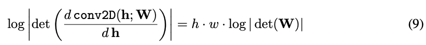
The log-determinant of an invertible 1 × 1 convolution of a h × w × c tensor
with c × c weight matrix W is straightforward to compute:
The cost of computing or differentiating det(W) is O(
), which is often comparable to the cost computing conv2D(h;W) which is O(h·W·
). We initialize the weights W as a random rotation matrix, having a log-determinant of 0; after one SGD step these values start to diverge from 0.
h × w × c 张量 与 c × c 权矩阵 W 的 1 × 1 可逆卷积的对数行列式计算起来很简单,公式 (9)。
计算或微分 det(W) 的成本是 O(),这通常与计算 conv2D(
;W) 的成本是 O(h·W·
) 相当。我们将权值 W 初始化为一个随机旋转矩阵,其对数行列式为0; 在一个 SGD 步骤之后,这些值开始从 0 发散。
# Invertible 1x1 conv
def invertible_1x1_conv(z, logdet, forward=True):
    # Shape
    h,w,c = z.shape[1:]
    # Sample a random orthogonal matrix to initialise weights
    w_init = np.linalg.qr(np.random.randn(c,c))[0]
    w = tf.get_variable("W", initializer=w_init)
    # Compute log determinant
    dlogdet = h * w * tf.log(abs(tf.matrix_determinant(w)))
    if forward:
        # Forward computation
        _w = tf.reshape(w, [1,1,c,c])
        z = tf.nn.conv2d(z, _w, [1,1,1,1], ’SAME’)
        logdet += dlogdet
        return z, logdet
    else:
        # Reverse computation
        _w = tf.matrix_inverse(w)
        _w = tf.reshape(_w, [1,1,c,c])
        z = tf.nn.conv2d(z, _w, [1,1,1,1], ’SAME’)
        logdet -= dlogdet
        return z, logdet
LU Decomposition
This cost of computing det(W) can be reduced from O(
where P is a permutation matrix, L is a lower triangular matrix with ones on the diagonal, U is an upper triangular matrix with zeros on the diagonal, and s is a vector. The log-determinant is then simply:
The difference in computational cost will become significant for large c, although for the networks in our experiments we did not measure a large difference in wallclock computation time.
In this parameterization, we initialize the parameters by first sampling a random rotation matrix W, then computing the corresponding value of P (which remains fixed) and the corresponding initial values of L and U and s (which are optimized).
LU 分解
计算 det(W) 的成本可以通过在其 LU 分解中直接参数化 W 而从 O() 降低到 O(c),式 (10)。
其中 P 是一个排列矩阵,L 是一个对角为 1 的下三角矩阵,U 是一个对角为 0 的上三角矩阵,s 是一个向量。log 行列式很简单,式 (11)。
对于 c 较大时,计算成本的差异将变得非常显著,而本文没有测量到 wallclock 计算时间的巨大差异。
在此参数化中,首先对一个随机旋转矩阵 W 进行采样,然后计算 P 的对应值 (保持不变) 以及 L、U 和 s 的对应初值 (优化) 来初始化参数。
3. Affine Coupling Layers
A powerful reversible transformation where the forward function, the reverse function and the logdeterminant are computationally efficient, is the affine coupling layer introduced in (Dinh et al., 2014, 2016). See Table 1. An additive coupling layer is a special case with s = 1 and a log-determinant of 0.
(Dinh et al., 2014, 2016) 中引入的仿射耦合层是一种强大的可逆变换,其中正向函数、反向函数和对数行列式计算效率很高。见表 1 所示。加性耦合层是 s = 1,对数行列式为 0 的特殊情况。

Zero initialization
We initialize the last convolution of each NN() with zeros, such that each affine coupling layer initially performs an identity function; we found that this helps training very deep networks.
零初始化
我们用零初始化每个 NN() 的最后一个卷积,使每个仿射耦合层最初执行一个恒等函数; 我们发现这有助于训练深度网络。
Split and concatenation
As in (Dinh et al., 2014), the split() function splits h the input tensor into two halves along the channel dimension, while the concat() operation performs the corresponding reverse operation: concatenation into a single tensor. In (Dinh et al., 2016), another type of split was introduced: along the spatial dimensions using a checkerboard pattern. In this work we only perform splits along the channel dimension, simplifying the overall architecture.
分裂和连接
如 (Dinh et al., 2014), split() 函数沿着通道维将输入张量分成两半,而 concat() 操作执行相应的反向操作: 将输入张量拼接成单个张量。在 (Dinh et al., 2016) 中,引入了另一种类型的分裂: 沿着空间维度使用棋盘模式。在这项工作中,我们只沿着通道维度进行分割,从而简化了整体架构。
Permutation
Each step of flow above should be preceded by some kind of permutation of the variables that ensures that after sufficient steps of flow, each dimensions can affect every other dimension. The type of permutation specifically done in (Dinh et al., 2014, 2016) is equivalent to simply reversing the ordering of the channels (features) before performing an additive coupling layer. An alternative is to perform a (fixed) random permutation. Our invertible 1x1 convolution is a generalization of such permutations. In experiments we compare these three choices.
排列
上述流程的每个步骤之前都应该有某种变量的排列,以确保在足够的流程步骤之后,每个维度都可以影响其他维度。在 (Dinh et al., 2014, 2016) 中具体完成的排列类型相当于在执行附加耦合层之前简单地反转通道 (特征) 的顺序。另一种方法是执行 (固定的) 随机排列。可逆 1x1 卷积是这种排列的推广。在实验中,我们比较了这三种选择。
Quantitative Experiments
We begin our experiments by comparing how our new flow compares against RealNVP (Dinh et al., 2016). We then apply our model on other standard datasets and compare log-likelihoods against previous generative models. See the appendix for optimization details. In our experiments, we let each NN() have three convolutional layers, where the two hidden layers have ReLU activation functions and 512 channels. The first and last convolutions are 3 × 3, while the center convolution is 1 × 1, since both its input and output have a large number of channels, in contrast with the first and last convolution.
我们通过比较 Glow 与 RealNVP (Dinh et al., 2016) 的对比来开始我们的实验。然后,将本文的模型应用于其他标准数据集,并将对数似然与之前的生成模型进行比较。有关优化细节,请参阅附录。本实验中,每个 NN() 有三个卷积层,其中两个隐藏层有 ReLU 激活函数和 512通道。第一和最后的卷积是 3 × 3,而中心卷积是 1 × 1,因为与第一和最后的卷积相比,其输入和输出都有大量的通道。

Gains using invertible 1 × 1 Convolution
We choose the architecture described in Section 3, and consider three variations for the permutation of the channel variables - a reversing operation as described in the RealNVP, a fixed random permutation, and our invertible 1 × 1 convolution. We compare for models with only additive coupling layers, and models with affine coupling. As described earlier, we initialize all models with a data-dependent initialization which normalizes the activations of each layer. All models were trained with K = 32 and L = 3. The model with 1 × 1 convolution has a negligible 0.2% larger amount of parameters.
我们选择第 3 节中描述的体系结构,并考虑信道变量排列的三种变化——RealNVP 中描述的反向操作、固定的随机排列和可逆的 1 × 1 卷积。我们比较了只有附加耦合层的模型和具有仿射耦合的模型。如前所述,我们使用依赖于数据的初始化来初始化所有模型,该初始化将每个层的激活规范化。所有模型的训练 K = 32, L = 3。具有 1 × 1 卷积的模型的参数量增加了 0.2%,可以忽略不计。
We compare the average negative log-likelihood (bits per dimension) on the CIFAR-10 (Krizhevsky, 2009) dataset, keeping all training conditions constant and averaging across three random seeds. The results are in Figure 3. As we see, for both additive and affine couplings, the invertible 1 × 1 convolution achieves a lower negative log likelihood and converges faster. The affine coupling models also converge faster than the additive coupling models. We noted that the increase in wallclock time for the invertible 1 × 1 convolution model was only ≈ 7%, thus the operation is computationally efficient as well.
我们比较了CIFAR-10 (Krizhevsky, 2009) 数据集上的平均负对数似然,保持所有训练条件不变,并在三个随机种子上进行平均。结果如图 3 所示。正如我们所看到的,对于加法和仿射耦合,可逆的 1 × 1 卷积实现了更低的负对数似然,收敛更快。仿射耦合模型也比加法耦合模型收敛速度快。我们注意到,对于可逆的 1 × 1 卷积模型,wallclock 时间的增加仅为 ≈7%,因此该操作的计算效率也很高。

Comparison with RealNVP on standard benchmarks
Besides the permutation operation, the RealNVP architecture has other differences such as the spatial coupling layers. In order to verify that our proposed architecture is overall competitive with the RealNVP architecture, we compare our models on various natural images datasets. In particular, we compare on CIFAR-10, ImageNet (Russakovsky et al., 2015) and LSUN (Yu et al., 2015) datasets. We follow the same preprocessing as in (Dinh et al., 2016). For Imagenet, we use the 32 × 32 and 64 × 64 downsampled version of ImageNet (Oord et al., 2016), and for LSUN we downsample to 96 × 96 and take random crops of 64 × 64. We also include the bits/dimension for our model trained on 256 × 256 CelebA HQ used in our qualitative experiments. As we see in Table 2, our model achieves a significant improvement on all the datasets.
除了排列操作之外,RealNVP 体系结构还有其他不同之处,比如空间耦合层。为了验证我们提出的体系结构与 RealNVP 体系结构的整体竞争力,我们在各种自然图像数据集上比较了我们的模型。特别地,我们比较了 CIFAR-10、ImageNet (Russakovsky et al., 2015) 和 LSUN (Yu et al., 2015) 数据集。我们遵循与 (Dinh et al., 2016) 相同的预处理。对于 Imagenet,我们使用 32 × 32 和 64 × 64 向下采样版本的 Imagenet (Oord et al., 2016),对于 LSUN,我们向下采样到96 × 96,并随机 crop 选取 64 × 64。我们还包括我们在定性实验中使用的 256 × 256 CelebA HQ 训练的模型的位/维正如我们在表 2 中看到的,我们的模型在所有数据集上取得了显著的改进。

Qualitative Experiments
We now study the qualitative aspects of the model on high-resolution datasets. We choose the CelebA-HQ dataset (Karras et al., 2017), which consists of 30000 high resolution images from the CelebA dataset, and train the same architecture as above but now for images at a resolution of 2562 , K = 32 and L = 6. To improve visual quality at the cost of slight decrease in color fidelity, we train our models on 5-bit images. We aim to study if our model can scale to high resolutions, produce realistic samples, and produce a meaningful latent space. Due to device memory constraints, at these resolutions we work with minibatch size 1 per PU, and use gradient checkpointing (Salimans and Bulatov, 2017). In the future, we could use a constant amount of memory independent of depth by utilizing the reversibility of the model (Gomez et al., 2017).
我们现在在高分辨率数据集上研究模型的定性方面。我们选择了CelebA- hq数据集,该数据集由来自 CelebA 数据集的 30000 张高分辨率图像组成,并训练了与上述相同的架构,但现在的图像分辨率为 2562, K = 32, L = 6。为了以略微降低色彩保真度为代价提高视觉质量,训练使用 5 位图像。我们的目标是研究我们的模型是否可以缩放到高分辨率,产生真实的样本,并产生有意义的潜在空间。由于设备内存限制,在这些分辨率下,我们使用每 PU 1 个 minibatch,并使用 gradient checkpointing。在未来,我们可以利用模型的可逆性,使用不依赖深度的恒定数量的记忆。
Consistent with earlier work on likelihood-based generative models (Parmar et al., 2018), we found that sampling from a reduced-temperature model often results in higher-quality samples. When sampling with temperature T, we sample from the distribution
. In case of additive coupling layers, this can be achieved simply by multiplying the standard deviation of pθ(z) by a factor of T.
与早期基于可能性的生成模型的研究一致,我们发现,从降温模型 (reduced-temperature model) 中取样通常会产生更高质量的样本。当温度为 T 时,从 分布中采样。对于附加耦合层,这可以简单地通过将 pθ(z) 的标准差乘以因子 T 来实现。
Synthesis and Interpolation
Figure 4 shows the random samples obtained from our model. The images are extremely high quality for a non-autoregressive likelihood based model. To see how well we can interpolate, we take a pair of real images, encode them with the encoder, and linearly interpolate between the latents to obtain samples. The results in Figure 5 show that the image manifold of the generator distribution is extremely smooth and almost all intermediate samples look like realistic faces.
图 4 显示了从我们的模型中得到的随机样本。对于非自回归似然模型来说,图像质量非常高。为了观察插值效果如何,我们取一对真实图像,用编码器对它们进行编码,并在潜伏期之间进行线性插值以获得样本。图 5 的结果表明,生成器分布的图像流形非常光滑,几乎所有的中间样本看起来都像真实的面孔。


Semantic Manipulation
We now consider modifying attributes of an image. To do so, we use the labels in the CelebA dataset. Each image has a binary label corresponding to presence or absence of attributes like smiling, blond hair, young, etc. This gives us 30000 binary labels for each attribute. We then calculate the average latent vector z_pos for images with the attribute and z_neg for images without, and then use the difference (z_pos − z_neg) as a direction for manipulating. Note that this is a relatively small amount of supervision, and is done after the model is trained (no labels were used while training), making it extremely easy to do for a variety of different target attributes. The results are shown in Figure 6.
现在我们考虑修改图像的属性。为此,我们使用了 CelebA 数据集中的标签。每个图像都有一个二进制标签,对应着微笑、金发、年轻等属性的存在或不存在。这为每个属性提供了 30000 个二进制标签。然后我们计算平均潜向量 z_pos 为图像与属性和 z_neg 为图像,然后使用差异 (z_pos - z_neg) 作为操作方向。注意,这是一个相对较少的监督,并且是在模型训练之后进行的 (在训练期间没有使用标签),这使得对各种不同的目标属性进行监督非常容易。结果如图 6 所示。

Effect of temperature and model depth
Figure 8 shows how the sample quality and diversity varies with temperature. The highest temperatures have noisy images, possibly due to overestimating the entropy of the data distribution, and thus we choose a temperature of 0.7 as a sweet spot for diversity and quality of samples. Figure 9 shows how model depth affects the ability of the model to learn long-range dependencies.
图 8 显示了样品质量和多样性随温度的变化情况。最高温度的图像有噪声,可能是由于高估了数据分布的熵,因此我们选择 0.7 的温度作为多样性和样本质量的最佳点。图 9 显示了模型深度如何影响模型学习长期依赖关系的能力。


Conclusion
We propose a new type of flow, coined Glow, and demonstrate improved quantitative performance in terms of log-likelihood on standard image modeling benchmarks. In addition, we demonstrate that when trained on high-resolution faces, our model is able to synthesize realistic images. Our model is, to the best of our knowledge, the first likelihood-based model in the literature that can efficiently synthesize high-resolution natural images.
我们提出了一种新的流类型,称为 Glow。
当训练高分辨率的面孔,我们的模型能够合成逼真的图像。
第一个基于似然,可以有效地合成高分辨率的自然图像的模型。