目录
论文名称:《Going Deeper with Convolutions》
code:
- (官方链接,TensorFlow):https://github.com/conan7882/GoogLeNet-Inception
- (另一个 PyTorch 版本,我觉得相对好理解一点的版本):https://github.com/Lornatang/GoogLeNet-PyTorch
写在前面
这篇文章的理论依据真的难懂!!!但有一说一,网络的设计还是挺不错的,能接受。
简介
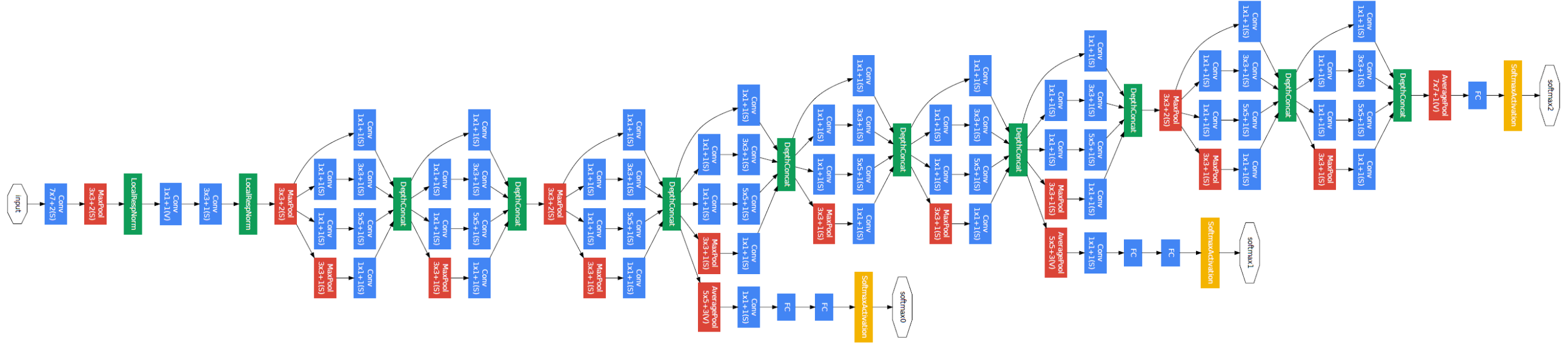
本篇文章提出了 Inception 结构,这样在增加模型的宽度(每一层的神经元个数)和深度时,计算量仍然可以接受。最后介绍了一下他们在 ILSVRC14 比赛上夺冠的网络结构 GoogLeNet,一个 22 层深的网络结构。
相关工作
这个部分一开始看的懵懵的,看是看得懂,但是不太明白为什么这么写。后来看完后面的网络设计再返回回来看这部分就恍然大明白了!(这告诉我们坚持下去就是胜利哈哈哈!)
- Serre et al. [15] 提出使用一系列固定但不同尺寸的 Gabor 滤波器来处理不用的缩放尺度。这就给文章提出 Inception 结构的启发:在每个 Inception 中 concatenate 1 × 1、3 × 3、5 × 5 的结果。与 [15] 相比的优势就是滤波器的参数都是模型自己学的。
- Lin et al. [12] 提出使用 1 × 1 的卷积层来增加模型的深度,以此增加模型的 representational power。文章在设计 Inception 结构,也用了这个 trick,两个目的:1、减少维度以减少计算量的瓶颈 2、增加模型的深度
- the Regions with Convolutional Neural Networks (R-CNN) [6] 是一个 two-stage 的检测模型:1、使用低层次的线索比如颜色、纹理来产生候选区域 2、使用 CNN 分类器识别候选区域中物体的种类。这样两阶段的方法就充分利用了低层次的线索,所以文章在设计 GoogleNet 也参考了这个 trick:在最后的分类结果中考虑低层次的信息,在靠近输入层的几个卷积层的输出(低层次信息)后,接一个简单的辅助网络(auxiliary network)来进行分类,其结果与模型最后的输出层一并 average 得到最后的结果。
动机 & High Level Consideration
这个标题的后半部分实在不知道怎么翻译了(我不够高级,不敢说话。。。)By the way,吐槽一下,这是整篇论文当中最没看懂的地方,第一次看的时候一边看一边心里边骂:“mmd,英语白学了!”(气哭.jpg),实在是看到火大,看了一半就被气到放一边去了(不怪大佬,怪我菜!)。第二天才鼓起勇气看完剩下的部分,剩下的部分很好理解。
我这里整理了一下我看懂的部分 以及 大牛们对这个部分的讲解。
先说说作者设计网络的动机:
提高网络的性能最简单粗暴的方法就是增加模型的深度和宽度,但这么做有两大 drawbacks:1、增加模型的深度和宽度,直接导致模型参数量更大, 如果数据还不够多,更容易过拟合 2、计算资源大大增加
作者提出的解决方案(同样也是理论基础,对,就是我没看懂的地儿。。。):将 dense 连接转换为为 sparse 稀疏连接
理解参考链接:
https://zhuanlan.zhihu.com/p/32702031(原创解释,下面的链接是根据这个链接的进一步总结)
https://zhuanlan.zhihu.com/p/69345065(下面这一部分内容主要参考这个链接里的内容)
稀疏连接
稀疏连接有两种方法:
- 空间(
spatial)上的稀疏连接,也就是 CNN。其只对输入图像的局部进行卷积,而不是对整个图像进行卷积,同时参数共享降低了总参数的数目并减少了计算量- 在特征(
feature)维度上的稀疏连接进行处理,也就是在通道的维度上进行处理。上面第二点,就是 Inception 结构的灵感来源。如果数据集的概率分布能够被一个大的稀疏神经网络进行表示,那么最优网络拓扑可以通过如下方式逐层构建:分析上一层的激活输出的统计特性,并将具有高度相关性输出的 filter 进行聚类(clustering),来获得一个稀疏的表示。
尽管严格的数学证明需要较强的条件,但是结合 Hebbian principle,实际上,即使在弱条件下,该论断也是成立的。
Hebbian Principe
Hebbian Principe 是一个很通俗的现象:先摇铃铛,之后给一只狗喂食,久而久之,狗听到铃铛就会口水连连。这时狗的听到铃铛的神经元与控制流口水的神经元之间的连接被加强了。
Hebbian Principe 的精确表达就是:如果两个神经元常常同时产生动作电位,或者说同时激活(
fire),这两个神经元之间的连接就会变强(neurons that fire together, wire together),反之则变弱。对应到神经网络的 filter bank,就是将强化具有相似特征的 filter 之间的关联。具体做法就是:用更少的 filter 来提取相关的特征,但是通过多个尺度的 filter bank 进行不相关的特征组合。实际上就是预先把相关性强的特征汇聚,就能起到加速收敛的作用。
稀疏矩阵的分解
举个例子,下图左侧是个稀疏矩阵(很多元素都为0,不均匀分布在矩阵中),和一个 2 x 2 的矩阵进行卷积,需要对稀疏矩阵中的每一个元素进行计算;如果像右图那样把稀疏矩阵分解成2个子密集矩阵,再和 2 x 2 矩阵进行卷积,稀疏矩阵中 0 较多的区域就可以不用计算,计算量就大大降低。
filter bank 的维度处理
上面系数矩阵对应到
Inception中,就是在通道维度上,将稀疏连接转换为密集连接。比方说 3 × 3 的卷积核,提取
256个特征,其总特征可能会均匀分散于每个feature map上,可以理解为一个稀疏连接的特征集。可以极端假设,64个filter提取的特征的密度,显然比256个filter提取的特征的密度要高。因此,通过使用 1 × 1,3 × 3,5 × 5 等,卷积核数分别为
96,96,64个,分别提取不同尺度的特征,并保持总的filter bank尺寸不变。这样,同一尺度下的特征之间的相关性更强,密度更大,而不同尺度的特征之间的相关性被弱化。综上所述,可以理解为将一个包含
256个均匀分布的特征,分解为了几组强相关性的特征组。同样是256个特征,但是其输出特征的冗余信息更少。(感觉有点儿类似于分组卷积)

结构细节

注意!这个图是从下往上看的!下面是输入,上面是输出。
- 3 × 3 和 5 × 5 卷积前的 1 × 1 卷积是用来减少维度,以此减少计算量的。
- Inception 结构是在模型的高层才出现,前几层还是传统的卷积层
实现代码(PyTorch)
class Inception(nn.Module):
    __constants__ = ['branch2', 'branch3', 'branch4']

    def __init__(self, in_channels, ch1x1, ch3x3red, ch3x3, ch5x5red, ch5x5, pool_proj,
                 conv_block=None):
        super(Inception, self).__init__()
        if conv_block is None:
            conv_block = BasicConv2d
        self.branch1 = conv_block(in_channels, ch1x1, kernel_size=1)

        self.branch2 = nn.Sequential(
            conv_block(in_channels, ch3x3red, kernel_size=1),
            conv_block(ch3x3red, ch3x3, kernel_size=3, padding=1)
        )

        self.branch3 = nn.Sequential(
            conv_block(in_channels, ch5x5red, kernel_size=1),
            conv_block(ch5x5red, ch5x5, kernel_size=3, padding=1)
        )

        self.branch4 = nn.Sequential(
            nn.MaxPool2d(kernel_size=3, stride=1, padding=1, ceil_mode=True),
            conv_block(in_channels, pool_proj, kernel_size=1)
        )

    def _forward(self, x):
        branch1 = self.branch1(x)
        branch2 = self.branch2(x)
        branch3 = self.branch3(x)
        branch4 = self.branch4(x)

        outputs = [branch1, branch2, branch3, branch4]
        return outputs

    def forward(self, x):
        outputs = self._forward(x)
        return torch.cat(outputs, 1)
GoogleNet

文章发现中间层的特征也非常 discriminative,所以在 Inception 4a 和 4d 的输出那里接出了一个 smaller convolutional networks。在训练过程中,这些 auxiliary network 的 loss 也以 0.3 的权重加到 total loss 中进行 auxiliary network 参数的更新。
auxiliary network architecture:
- An average pooling layer with 5×5 filter size and stride 3
- A 1×1 convolution with 128 filters for dimension reduction and rectified linear activation
- A fully connected layer with 1024 units and rectified linear activation
- A dropout layer with 70% ratio of dropped outputs
- A linear layer with softmax loss as the classifier (predicting the same 1000 classes as the main classifier, but removed at inference time)

实现代码(PyTorch)
我放出来的有删减,只放出了最核心的部分。完整版参考链接:https://github.com/Lornatang/GoogLeNet-PyTorch/blob/772dd5ff866c0ba26ecce5a89e5839654510b185/googlenet_pytorch/model.py#L39
class GoogLeNet(nn.Module):
    __constants__ = ['aux_logits', 'transform_input']

    def __init__(self, global_params=None):
        super(GoogLeNet, self).__init__()

        if global_params.blocks is None:
            blocks = [BasicConv2d, Inception, InceptionAux]
        assert len(blocks) == 3
        conv_block = blocks[0]
        inception_block = blocks[1]
        inception_aux_block = blocks[2]

        self.aux_logits = global_params.aux_logits
        self.transform_input = global_params.transform_input

        self.conv1 = conv_block(3, 64, kernel_size=7, stride=2, padding=3)
        self.maxpool1 = nn.MaxPool2d(3, stride=2, ceil_mode=True)
        self.conv2 = conv_block(64, 64, kernel_size=1)
        self.conv3 = conv_block(64, 192, kernel_size=3, padding=1)
        self.maxpool2 = nn.MaxPool2d(3, stride=2, ceil_mode=True)

        self.inception3a = inception_block(192, 64, 96, 128, 16, 32, 32)
        self.inception3b = inception_block(256, 128, 128, 192, 32, 96, 64)
        self.maxpool3 = nn.MaxPool2d(3, stride=2, ceil_mode=True)

        self.inception4a = inception_block(480, 192, 96, 208, 16, 48, 64)
        self.inception4b = inception_block(512, 160, 112, 224, 24, 64, 64)
        self.inception4c = inception_block(512, 128, 128, 256, 24, 64, 64)
        self.inception4d = inception_block(512, 112, 144, 288, 32, 64, 64)
        self.inception4e = inception_block(528, 256, 160, 320, 32, 128, 128)
        self.maxpool4 = nn.MaxPool2d(2, stride=2, ceil_mode=True)

        self.inception5a = inception_block(832, 256, 160, 320, 32, 128, 128)
        self.inception5b = inception_block(832, 384, 192, 384, 48, 128, 128)

        if global_params.aux_logits:
            self.aux1 = inception_aux_block(512, global_params.num_classes)
            self.aux2 = inception_aux_block(528, global_params.num_classes)

        self.avgpool = nn.AdaptiveAvgPool2d((1, 1))
        self.dropout = nn.Dropout(p=global_params.dropout_rate)
        self.fc = nn.Linear(1024, global_params.num_classes)

        for m in self.modules():
            if isinstance(m, nn.Conv2d):
                nn.init.kaiming_normal_(m.weight, mode='fan_out', nonlinearity='relu')
                if m.bias is not None:
                    nn.init.constant_(m.bias, 0)
            elif isinstance(m, nn.BatchNorm2d):
                nn.init.constant_(m.weight, 1)
                nn.init.constant_(m.bias, 0)
            elif isinstance(m, nn.Linear):
                nn.init.normal_(m.weight, 0, 0.01)
                nn.init.constant_(m.bias, 0)


    def _forward(self, x):
        # type: (Tensor) -> Tuple[Tensor, Optional[Tensor], Optional[Tensor]]
        # N x 3 x 224 x 224
        x = self.conv1(x)
        # N x 64 x 112 x 112
        x = self.maxpool1(x)
        # N x 64 x 56 x 56
        x = self.conv2(x)
        # N x 64 x 56 x 56
        x = self.conv3(x)
        # N x 192 x 56 x 56
        x = self.maxpool2(x)

        # N x 192 x 28 x 28
        x = self.inception3a(x)
        # N x 256 x 28 x 28
        x = self.inception3b(x)
        # N x 480 x 28 x 28
        x = self.maxpool3(x)
        # N x 480 x 14 x 14
        x = self.inception4a(x)
        # N x 512 x 14 x 14
        aux_defined = self.training and self.aux_logits
        if aux_defined:
            aux1 = self.aux1(x)
        else:
            aux1 = None

        x = self.inception4b(x)
        # N x 512 x 14 x 14
        x = self.inception4c(x)
        # N x 512 x 14 x 14
        x = self.inception4d(x)
        # N x 528 x 14 x 14
        if aux_defined:
            aux2 = self.aux2(x)
        else:
            aux2 = None

        x = self.inception4e(x)
        # N x 832 x 14 x 14
        x = self.maxpool4(x)
        # N x 832 x 7 x 7
        x = self.inception5a(x)
        # N x 832 x 7 x 7
        x = self.inception5b(x)
        # N x 1024 x 7 x 7

        x = self.avgpool(x)
        # N x 1024 x 1 x 1
        x = torch.flatten(x, 1)
        # N x 1024
        x = self.dropout(x)
        x = self.fc(x)
        # N x 1000 (num_classes)
        return x, aux2, aux1


    def forward(self, x):
        # type: (Tensor) -> GoogLeNetOutputs
        x = self._transform_input(x)
        x, aux1, aux2 = self._forward(x)
        aux_defined = self.training and self.aux_logits
        if torch.jit.is_scripting():
            if not aux_defined:
                warnings.warn("Scripted GoogleNet always returns GoogleNetOutputs Tuple")
            return GoogLeNetOutputs(x, aux2, aux1)
        else:
            return self.eager_outputs(x, aux2, aux1)
训练技巧
值得特别注意的两个数据增强的技巧:
- sampling of various sized patches of the image whose size is distributed evenly between 8% and 100% of the image area with aspect ratio constrained to the interval [ 3/4 , 4/3 ].
- photometric distortions of Andrew Howard [8](待了解)
ILSVRC 2014 分类任务的结果

测试技巧
- independently trained 7 versions of the same GoogLeNet model (including one wider version), and performed ensemble prediction with them. These models were trained with the same initialization (even with the same initial weights, due to an oversight) and learning rate policies. They differed only in sampling methodologies and the randomized input image order.
- adopted a more aggressive cropping approach(This leads to 4×3×6×2 = 144 crops per image.):
- resized the image to 4 scales where the shorter dimension (height or width) is 256, 288, 320 and 352 respectively【公式中的 4】
- take the left, center and right square of these resized images (in the case of portrait images, we take the top, center and bottom squares)【公式中的 3】
- For each square, we then take the 4 corners and the center 224×224 crop as well as the square resized to 224×224, and their mirrored versions. 【公式中的 (4 + 1 + 1) * 2】
- The softmax probabilities are averaged over multiple crops and over all the individual classifiers to obtain the final prediction.
Things To Learn
- photometric distortions 【8】