波士顿房价预测

import numpy as np
import matplotlib as mpl
import matplotlib.pyplot as plt
from sklearn.model_selection import train_test_split
from sklearn.linear_model import ElasticNetCV
import sklearn.datasets
from pprint import pprint
from sklearn.preprocessing import PolynomialFeatures, StandardScaler
from sklearn.pipeline import Pipeline
from sklearn.metrics import mean_squared_error
from sklearn.ensemble import RandomForestRegressor
import warnings
def not_empty(s):
    return s != ''
if __name__ == "__main__":
    data = sklearn.datasets.load_boston()
    x = np.array(data.data)
    y = np.array(data.target)
    print('样本个数：%d, 特征个数：%d' % x.shape)
    print(y.shape)
    y = y.ravel()

    x_train, x_test, y_train, y_test = train_test_split(x, y, train_size=0.7, random_state=0)
    model = Pipeline([
        ('ss', StandardScaler()),
        ('poly', PolynomialFeatures(degree=3, include_bias=True)),
        ('linear', ElasticNetCV(l1_ratio=[0.1, 0.3, 0.5, 0.7, 0.99, 1], alphas=np.logspace(-3, 2, 5),
                                fit_intercept=False, max_iter=1e3, cv=3))
    ])
    # model = RandomForestRegressor(n_estimators=50, criterion='mse')
    print('开始建模...')
    model.fit(x_train, y_train)
    linear = model.get_params('linear')['linear']
    print(u'超参数：', linear.alpha_)
    print(u'L1 ratio：', linear.l1_ratio_)
    print(u'系数：', linear.coef_.ravel())

    order = y_test.argsort(axis=0)
    y_test = y_test[order]
    x_test = x_test[order, :]
    y_pred = model.predict(x_test)
    r2 = model.score(x_test, y_test)
    mse = mean_squared_error(y_test, y_pred)
    print('R2:', r2)
    print('均方误差：', mse)

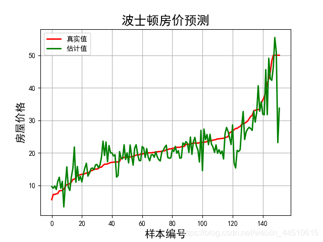
    t = np.arange(len(y_pred))
    mpl.rcParams['font.sans-serif'] = ['simHei']
    mpl.rcParams['axes.unicode_minus'] = False
    plt.figure(facecolor='w')
    plt.plot(t, y_test, 'r-', lw=2, label='真实值')
    plt.plot(t, y_pred, 'g-', lw=2, label='估计值')
    plt.legend(loc='best')
    plt.title('波士顿房价预测', fontsize=18)
    plt.xlabel('样本编号', fontsize=15)
    plt.ylabel('房屋价格', fontsize=15)
    plt.grid()
    plt.show()

超参数： 0.31622776601683794
L1 ratio： 0.99
R2: 0.7722034192609936
均方误差： 18.967596568189173

使用RandomForestRegressor

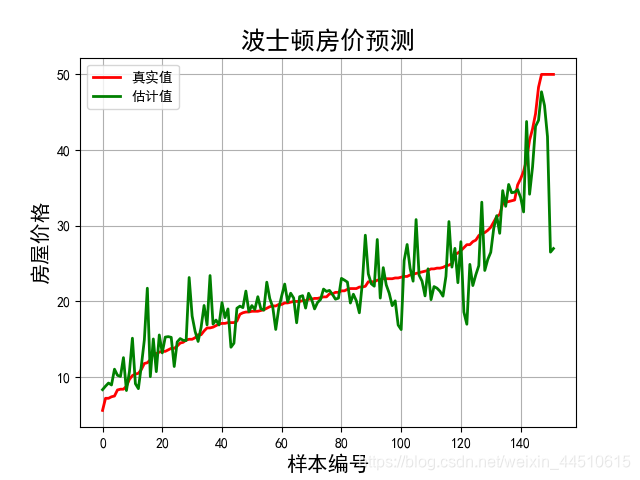
R2: 0.7986958266918252
均方误差： 16.761692973684216