Chapter 2:Discrete-Time Signals in The Time Domain

Time-Domain Representation

Signals represented as sequences of numbers,called samples

Sample value of a typical signal or sequence denoted as x[n] with n being an integer in the range $-\infty ⩽n⩽\infty$

x[n] defined only for integer values of n and undefined for noninteger values of n

Discrete-time signal represented by {x[n]}

Discrete-time signal may also be written as a sequence of numbers inside braces:

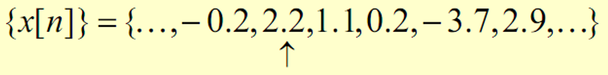
In the above,x[-1]=-0.2,x[0]=2.2,x[1]=1.1

The arrow is placed under the sample at time index n=0

Graphical representation of a discrete-time signal with real-time samples is as shown below:

In some applications, a discrete-time sequence {x[n]} may be generated by periodically sampling a continuous-time signal $x_{\alpha }(t)$ at uniform intervals of time

Here, n-th sample is given by
$x[n]=x_{\alpha }(t){|}_{t=nT}=x_{\alpha }(nT),n=\dots ，-2，-1，0，1，\dots$

The spacing T between two consecutive samples is called the sampling interval or sampling period

Reciprocal of sampling interval T，denoted as $F_T$, is called the sampling frequency:$F_T=\frac{1}{T}$

{x[n]} is a real sequence, if the n-th sample x[n] is real for all values of n

Otherwise, {x[n]} is a complex sequence

A complex sequence {x[n]} can be written as {x[n]}={xre[n]}+j{xim[n]} where xre[n] and xim[n] are the real and imaginary parts of x[n]

The complex conjugate sequence of {x[n]} is given by {x*[n]}={xre[n]}-j{xim[n]}

Length of a Discrete-Time Signal

A discrete-time signal may be a finite-length or an infinite-length sequence

Finite-length (also called finite-duration or finite-extent) sequence is defined only for a finite time interval:$N_1⩽n⩽N_2$ where $-\infty <N_1$ and $N_2<\infty$ with $N1⩽N_2$

Length or duration of the above finite-length sequence is $N=N_2-N_1+1$

A length-N sequence is often refered to as an N-point sequence

The length of a finite-length sequence can be increased by zero-padding

A right-sided sequence x[n] has zero-valued samples for $n<N_1$

If $N_1⩾0$，a right-sided sequence is called a causal sequence

A left-sided sequence x[n] has zero-valued samples for $n>N_2$

If $N_2⩽0$，a left-sided sequence is called a anti-causal sequence

Operations on Sequences

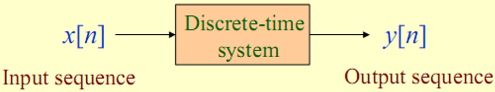
For example, the input may be a signal corrupted with additive noise

Discrete-time system is designed to generate an output by removing the noise component from the input

In most cases, the operation defining a particular discrete-time system is composed of some basic operations

Elementary Operations

Product (modulation) operation:

Addition operation:

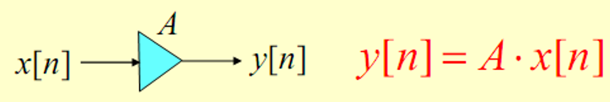
Multiplication operation:

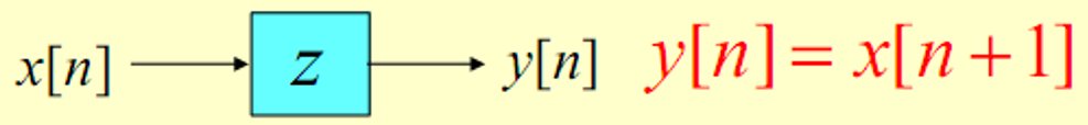
Time-shifting operation:$y[n]=x[n-N]$，where N is an interger

If N>0，it is delaying operation

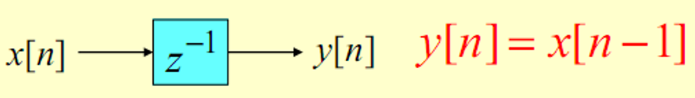
If N<0，it is an advance operation

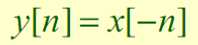
Time-reversal(folding) operation:

Branching operation: Used to provide multiple copies of a sequence

operations on two or more sequences can be carried out if all sequences involved are of same length and defined for the same range of the time index n

However if the sequences are not of same length, in some situations, this problem can be circumvented by appending zero-valued samples to the sequence(s) of smaller lengths to make all sequences have the same range of the time index

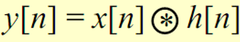
Convolution Sum

The summation $y[n]={\sum }_{k=-\infty }^{\infty }x[k]h[n-k]={\sum }_{k=-\infty }^{\infty }x[n-k]h[k]$ is called the convolution sum of the sequences x[n] and h[n] and represented comopactly as

In the example considered the convolution of a sequence {x[n]} of length 5 with a sequence {h[n]} of length 4 resulted in a sequence {y[n]} of length 8

In general, if the lengths of the two sequences being convolved are M and N，then the sequence generated by the convolution is of length M+N-1

Operations on Finite-Length Sequences

Circular Time-Reversal Operations

Modulo operaton：
$<m{>}_n=m(module)N$
Circular Time-Reversal Operations：
$y[n]=x[<-n{>}_N]$

Circular Shift of a Sequence

If x[n] is such a sequence, then for any arbitrary integer $n_o$，the shifted sequence $x_1[n]=x[n-n_o]$ is no longer defined for the range $0⩽n⩽N-1$

We thus need to define another type of a shift that will always keep the shiifted sequence in the range $0⩽n⩽N-1$

The desired shift, called the circular shift, is defined using a modulo operation:$x_c[n]=x[<n-n_o{>}_N]$

For $n_o>0$(right circular shift)，the above equation implies
$x_c[n]\{\begin{array}{c}x[n-n_o],for{n}_o⩽n⩽N-1\\ x[N-n_o+n],for0⩽n<N-1\end{array}$

a right circular shift by $n_o$ is equivalent to a left circular shift by $N-n_o$ sample periods

A circular shift by an integer number $n_o$ greater than N is equivalent to a circular shift by $<n_o{>}_N$

Classification of Sequences Based on Symmetry

Conjugate-symmetric sequence:
$x[n]=x^{\ast }[-n]$
If x[n] is real, then it is an even sequence

Conjugate-antisymmetric sequence:
$x[n]=-x^{\ast }[-n]$
If x[n] is real, then it is an odd sequence

It follows from the definition that for a conjugate-symmetric sequence {x[n]}，x[0] must be a real number

Likewise, it follows from the definition that for a conjugate anti-symmetric sequence {y[n]},y[0] must be an imaginary number

From the above, it also follows that for an odd sequence {w[n]},w[0] = 0

Any complex sequence can be expressed as a sum of its conjugate-symmetric part and its conjugate-antisymmetric part:
$x[n]=x_{cs}[n]+x_{ca}[n]$
where
$x_{cs}=\frac{1}{2}(x[n]+x^{\ast }[-n])$
$x_{ca}=\frac{1}{2}(x[n]-x^{\ast }[-n])$

Total energy of a sequence x[n] is defined by$\xi ={\sum }_{n=-\infty }^{\infty }|x[n]{|}^2$

The average power of an aperiodic sequence is defined by $P_x={\lim }_{K\to \infty }\frac{1}{2K+1}{\sum }_{n=-K}^K|x[n]{|}^2$

An infinite energy signal with finite average power is called a power signal

A finite energy signal with zero average power is called an energy signal

A sequence x[n] is said to be bounded if $|x[n]|⩽B_x<\infty$

Typical Sequences and Sequence Representation

Some Basic Sequences

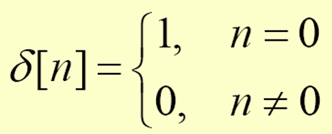
Unit sample sequence

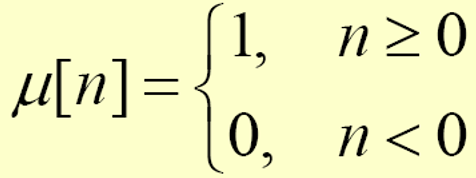
Unit step sequence

Real sinusoidal sequence
$x[n]=Acos({\omega }_{o}n+\varphi )$
where A is the amplitude，${\omega }_o$ is the angular frequency, and $\varphi$ is the phase of x[n]

Real exponential sequence
$x[n]=A{\alpha }^n，-\infty <n<\infty$
where A and $\alpha$ are real numbers

Sinusoidal sequence $Acos({\omega }_{o}n+\varphi )$ and complex exponential sequence $Bexp(j{\omega }_{o}n)$ are periodic sequences of period N if ${\omega }_{o}N=2\pi r$ where N and r are positive integers

Smallest value of N satisfying ${\omega }_{o}N=2\pi r$ is the fundamental period of the sequence

Representation of an Arbitrary Sequences

An arbitrary sequence can be represented in the time-domain as a weighted sum of some basic sequence and its delayed(advanced) versions

The Sampling Process

Often, a discrete-time sequence x[n] is developed by uniformly sampling a continuous-time signal $x_{\alpha }(t)$ as indicated below

The relation between the two signals is $x[n]=x_{\alpha }(t){|}_{t=nT}=x_{\alpha }(nT)，n=\dots ，-2，-1，0，1，2，\dots$

Time variable t of $x_{\alpha }(t)$ is related to the time variable n of x[n] only at discrete-time instants $t_n$ given by $t_n=nT=\frac{n}{F_T}=\frac{2\pi n}{{\Omega }_T}$ with $F_T=1/T$ denoting the sampling frequency and ${\Omega }_T=2\pi F_T$ denoting the sampling sampling angular frequency

Consider the continuous-time signal $x(t)=Acos(2\pi f_{o}t+\varphi )=Acos({\Omega }_{o}t+\varphi )$
The corresponding discrete-time signal is $x[n]=Acos({\Omega }_{o}nT+\varphi )=Acos(\frac{2\pi {\Omega }_o}{{\Omega }_T}n+\varphi )=Acos({\omega }_{o}n+\varphi )$
where ${\omega }_o=\frac{2\pi {\Omega }_o}{{\Omega }_T}={\Omega }_{o}T$ is the normalized digital angualr frequency of x[n]

If the unit of sampling period T is in seconds
The unit of normalized digital angualar frequency ${\omega }_o$ is radians/sample
The unit of normalized analog angualr frequency ${\Omega }_o$ is radians/second
The unit of analog frequency $f_o$ is herts(Hz)

Reference

1.《Digital Signal Processing：A Computer-Based Approach》