Chapter 3:Discrete-Time Signals in the Frequency Domain

The Discrete-Time Fourier Transform

Definition - The CTFT of a continuous-time signal $x_a(t)$ is given by
$X_a(j\Omega )={\int }_{-\infty }^{\infty }{x}_a(t)e^{-j\Omega t}dx$
Often referred to as the Fourier spectrum or simply the spectrum of the continuous-time signal

Definition - The inverse CTFT of a Fourier transform $X_a(j\Omega )$ is given by
$x_a(t)=\frac{1}{2\pi }{\int }_{-\infty }^{\infty }{X}_a(j\Omega )e^{j\Omega t}d\Omega$
Often referred to as the Fourier intergral

A CTFT pair will be denoted as
$x_a(t)\leftrightarrow X_a(j\Omega )$

Definition - The discrete-time Fourier transform (DTFT) $X(e^{jw})$ of a sequence x[n] is given by $X(e^{jw})={\sum }_{n=-\infty }^{\infty }x[n]e^{-jwn}$

$X(e^{jw})$ can alternately be expressed as $X(e^{jw})=|X(e^{jw})|e^{j\theta (\omega )}$，where $\theta (\omega )=arg\left\{X(e^{jw})\right\}$

$|X(e^{jw})|$ is called the magnitude function
$\theta (\omega )$ is called the phase function

Both quantities are again real functions of $w$

In many applications, the DTFT is called the Fourier spectrum

Likewise,$|X(e^{jw})|$ and $\theta (\omega )$ are called the magnitude and phase spectra

$X(e^{jw})=X_{re}(e^{jw})+j{X}_{im}(e^{jw})$
where:$X_{re}(e^{jw})=\frac{1}{2}(X(e^{jw})+X^{\ast }(e^{jw}))$ ---- real part
$X_{im}(e^{jw})=\frac{1}{2j}(X(e^{jw})-X^{\ast }(e^{jw}))$ ---- imaginary part

For a real sequence x[n],$|X(e^{jw})|$ and $X_{re}(e^{jw})$ are even functions of $w$，whereas，$\theta (\omega )$ and $X_{im}(e^{jw})$ are odd functions of $w$

Note: $X(e^{jw})=|X(e^{jw})|e^{j[q(w)+2pk]}=|X(e^{jw})|e^{j\theta (\omega )}$ for any integer k

The phase function $\theta (\omega )$ cannot be uniquely sepcified for any DTFT

Unless otherwise stated, we shall assume that the phase function $\theta (\omega )$ is restricted to the following range of values:$-\pi ⩽\theta (\omega )<\pi$ called the principal value

The DTFT $X(e^{jw})$ of a sequence $x[n]$ is a continuous function of $w$
It is also a periodic function of $w$ with a period $2\pi$

Therefore $X(e^{jw})={\sum }_{n=-\infty }^{\infty }x[n]e^{-jwn}$ represents the Fourier series representation of the periodic function

As a result, the Fourier coefficients x[n] can be computed from $X(e^{j\omega })$ using the Fourier integral $x[n]=\frac{1}{2\pi }{\int }_{-\pi }^{\pi }X(e^{j\omega })e^{j\omega n}d\omega$
Inverse discrete-time Fourier transform

Symmetry Relations of DTFT

DTFT Properties:Symmetry Relations

x[n]: A complex sequence

x[n]: A real sequence

Discrete-Time Fourier Transform Theorems

There are a number of important properties of the DTFT that are useful in signal processing applications

Table 3.4

An important property of the DTFT is given by the convolution theorem in Table 3.4
It states that if $y[n]=x[n]⊛h[n]$，then the DTFT $Y(e^{j\omega })$ of y[n] is given by $Y(e^{j\omega })=X(e^{j\omega })\ast H(e^{j\omega })$
An implication of this result is that the linear convolution y[n] of the sequences x[n] and h[n] can be performed as follows:

1. Compute the DTFTs $X(e^{j\omega })$ and $H(e^{j\omega })$ of the sequences x[n] and h[n]，respectively
2. Form the DTFT $Y(e^{j\omega })=X(e^{j\omega })H(e^{j\omega })$
3. Compute the IDFT y[n] of $Y(e^{j\omega })$

Digital Processing of Continuous-Time Signals

Digital processing of a continuous-time signal involves the following basic steps:

1. Conversion of the continuous-time signal into a discrete-time signal
2. Processing of the discrete-time signal
3. Conversion of the processed discrete-time signal back into a continuous-time signal

Conversion of a continuous-time signal into digital form is carried out by an analog-to-digital(A/D) converter

The reverse operation of converting a digital signal into a continuous-time signal is performed by a digital-to-analog(D/A) converter

Since the A/D conversion takes a finite amount of time, a sample-and-hold(S/H) circuit is used to ensure that the analog signal at the input of the A/D converter remains constant in amplitude until the conversion is complete to minimize the error in its representation

To prevent aliasing, an anti-aliasing filter is employed before the S/H circuit

To smooth the output signal of the D/A converter, which has a staircase-like waveform, an analog reconstruction filter is uesd.

Complete block-diagram

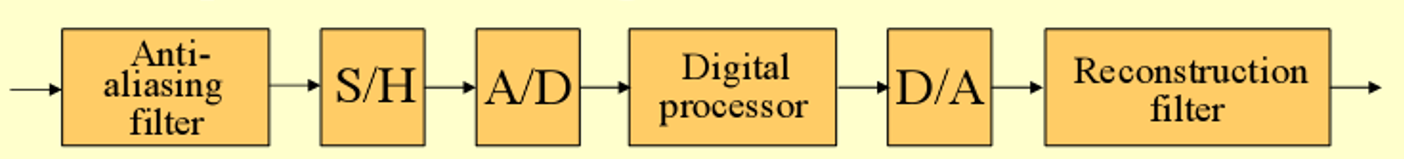
Since both the anti-aliasing filter and the reconstruction filter are analog lowpass filters, we review first the theory behind the design of such filters

Let $g_a(t)$ be a continuous-time signal that is sampled uniformly at t=nT，generating the sequence g[n] where $g[n]=g_a(nT)-\infty <n<\infty$ with T being the sampling period

The reciprocal of T is called the sampling frequency $F_T$，$F_T=\frac{1}{T}$

Now, the frequency-domain representation of $g_a(t)$ is given by its continuous-time Fourier transform(CTFT) ：$G_a(j\Omega )={\int }_{-\infty }^{\infty }{g}_a(t)e^{-j\Omega t}dt$

The frequency-domain representation of g[n] is given by its discrete-time Fourier transform (DTFT)：$G(e^{jw})={\sum }_{n=-\infty }^{\infty }g[n]e^{-jwn}$

To establish the relation between $G_a(j\Omega )$ and $G(e^{jw})$，we treat the sampling operation mathematically as a multiplication of $g_a(t)$ by a periodic impulse train p(t):
$p(t)={\sum }_{n=-\infty }^{\infty }\delta (t-nT)$

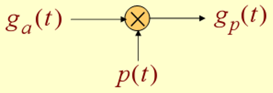
p(t) consists of a train of ideal impulse with a period T as shown below

The multiplication operation yields an impulse train:
$g_p(t)=g_a(t)p(t)={\sum }_{n=-\infty }^{\infty }{g}_a(nT)\delta (t-nT)$

$g_p(t)$ is a continuous-time signal consisting of a train of uniformly spaced impulse with the impluse at $t=nT$ weighted by the sampled value $g_a(nT)$ of $g_a(t)$ at that instant


There are two different forms of $G_p(j\Omega )$

One form is given by the weighted sum of the CTFTs of $\delta (t-nT)$：$G_p(j\Omega )={\sum }_{n=-\infty }^{\infty }{g}_a(nT)e^{-j\Omega nT}$

Assume $g_a(t)$ is band-limited signal with a CTFT $G_a(j\Omega )$ as shown below

The spectrum $P(j\Omega )$ of p(t) having a smpling period $T=\frac{2\pi }{{\Omega }_T}$ is indicated below

Two possible spectra of $G_p(j\Omega )$ are shown below


It is evident from the top figure on the previous slide that if ${\Omega }_T>2{\Omega }_m$，there is no overlap betweeen the shifted replicas of $G_a(j\Omega )$ generating $G_p(j\Omega )$

On the other hand, as indicated by the figure on the bottom, if ${\Omega }_T<2{\Omega }_m$，there is an overlap of the spectra of the shifted replicas of $G_a(j\Omega )$ generating $G_p(j\Omega )$

if ${\Omega }_T>2{\Omega }_m$，$g_a(t)$ can be recovered exactly from $g_p(t)$ by passing it through an ideal lowpass filter $H_r(j\Omega )$ with a gain T and a cutoff frequency ${\Omega }_c$ greater than ${\Omega }_m$ and less than ${\Omega }_T-{\Omega }_m$ as shown below


On the other hand, if ${\Omega }_T<2{\Omega }_m$，due to the overlap of the shifted replicas of $G_a(j\Omega )$，the spectrum $G_a(j\Omega )$ cannot be separated by filtering to recover $G_a(j\Omega )$ because of the distortion caused by a part of the replicas immediately outside the basedband folded back or aliased into the baseband.

Smpling theorem Let $g_a(t)$ be a band-limited signal with CTFT $G_a(j\Omega )=0$ for $|\Omega |>{\Omega }_m$

Then $g_a(t)$ is uniquely determined by its samples $g_a(nT)$,$-\infty ⩽n⩽\infty$ of ${\Omega }_T⩾2{\Omega }_m$ where ${\Omega }_T=2\pi /T$

The condition ${\Omega }_T⩾2{\Omega }_m$ is often referred to as the Nyquist condition

The frequency $\frac{{\Omega }_T}{2}$ is usually referred to as the folding frequency

The highest frequency ${\Omega }_m$ contained in $g_a(t)$ is usually called the Nyquist frequency since it determines the minimum sampling frequency ${\Omega }_T=2{\Omega }_m$ that must be used to fully recover $g_a(t)$ from its sampled version

The frequency $2{\Omega }_m$ is called the Nyquist rate

Oversampling - The sampling frequency is higher than the Nyquist rate
Undersampling - The sampling frequency is lower than the Nyquist rate
Critical sampling - The sampling frequency is equal to the Nyquist rate

Note: A pure sinusoid may not be recoverable from its critically sampled version

Reference

1.《Digital Signal Processing：A Computer-Based Approach》