文章目录
引言
matplotlib是一个用于生成图表的包,目的在于在python环境下进行MATLAB风格的绘图。seaborn是一个使用matplotlib进行底层绘图的附加工具包。
7.1matplotlib绘图
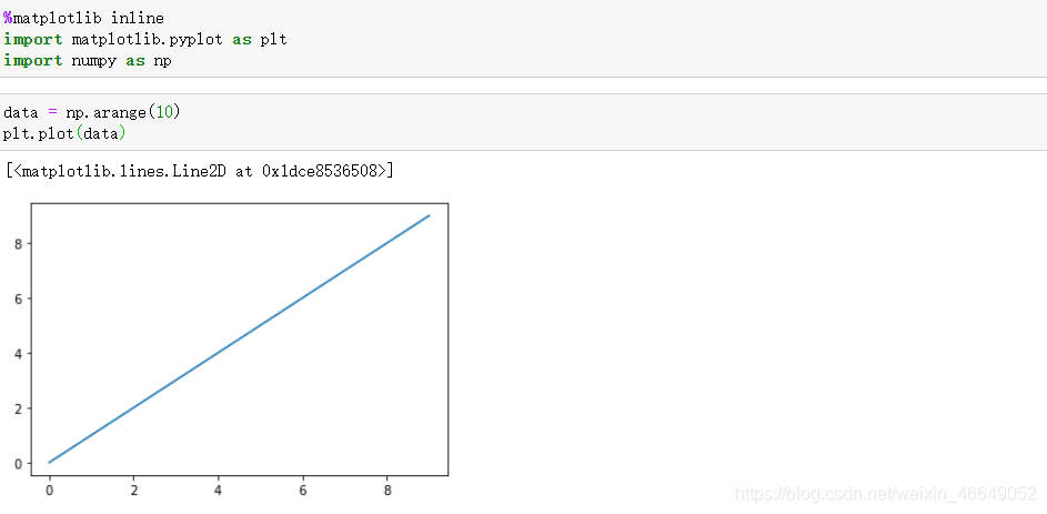
生成一个简单的图形
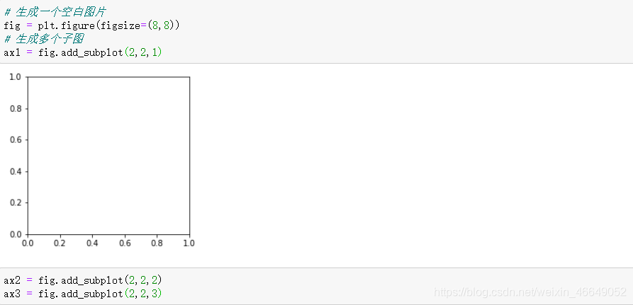
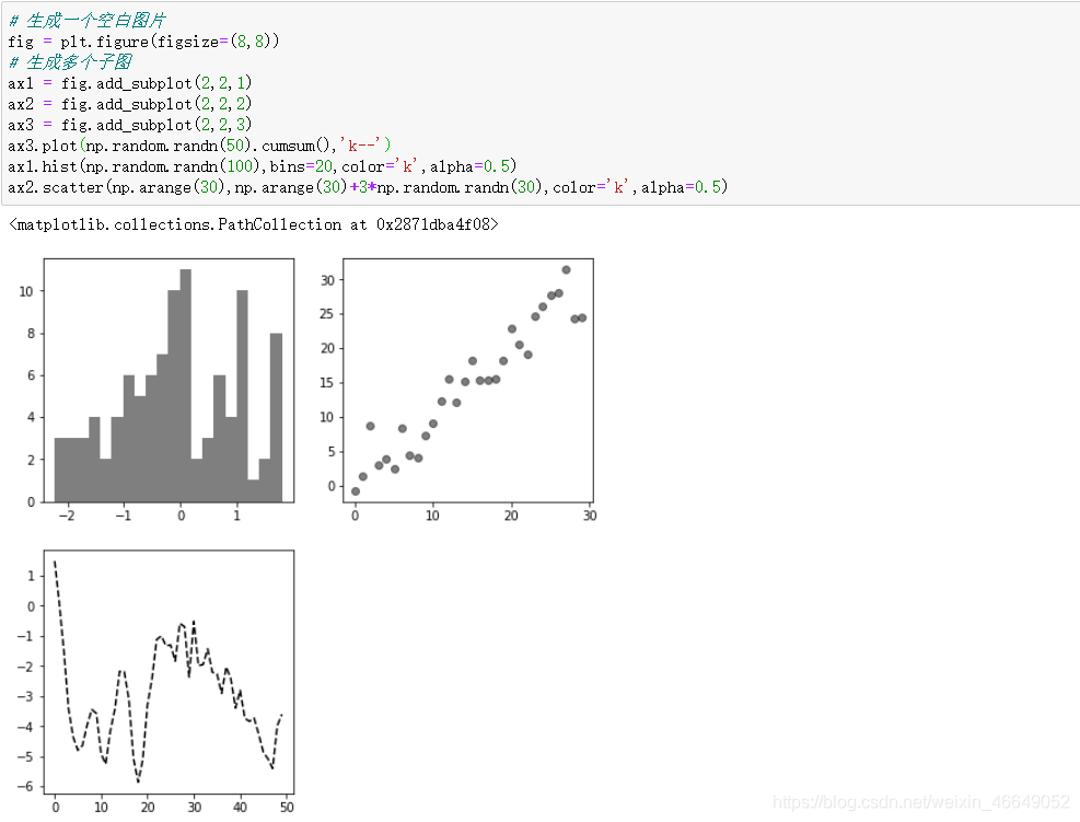
7.1.1 图片与子图
plt.figure()生成一个空白图片,figsize设置图片的大小,想要在空白图片上进行绘图,使用add_subplot()创建一个或多个子图。

注意:由于在每个单元格运行后,图标会被重置。所以对于复杂图表,需要将所有绘图命令放在单个notebook中。
子图的绘制:
matplotlib包含一个便捷方法plt.subplots,它创建一个新图片,并返回包含已生成子图对象的Numpy数组。
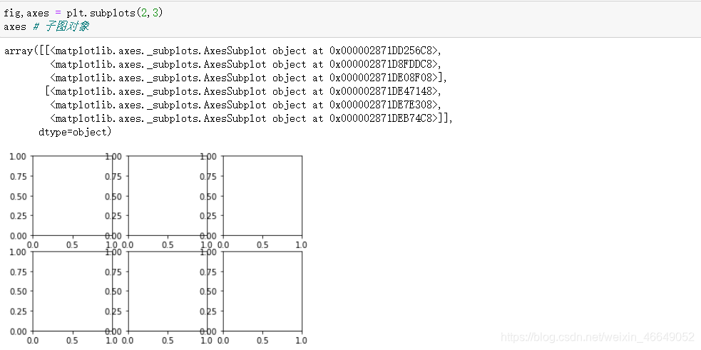
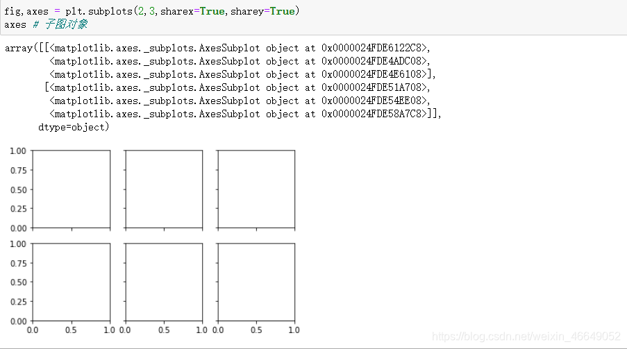
数组axes可以像二维数组那样方便索引,例如axes[0,1]。也可以通过参数sharex和sharey表明子图分别拥有相同的x轴与y轴,方便在相同比例下进行数据对比。
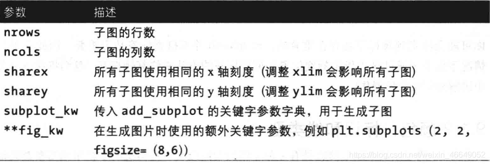
pyplot.subplots参数:
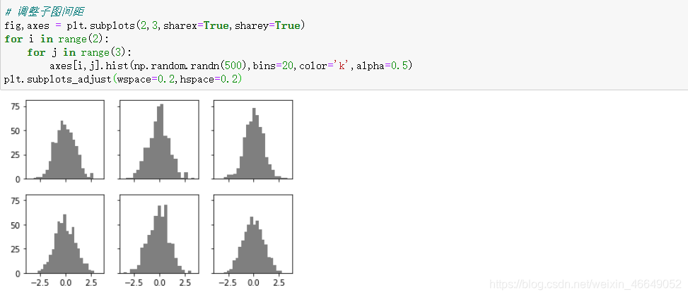
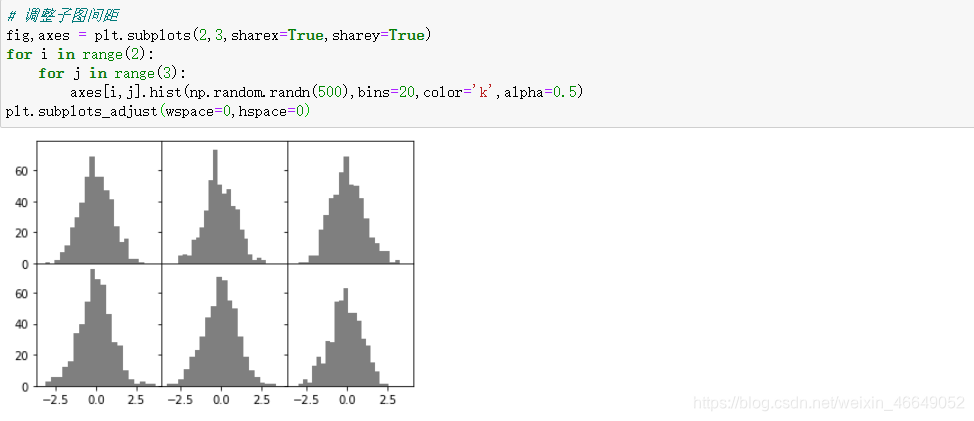
7.1.1调整子图周围的间距
使用图对象上的subplots_adjust方法来调整子图间距

前四个参数分别控制子图的左右上下边距,wspace和hspace分别控制图片的宽度与高度百分比,以用作子图间的间距
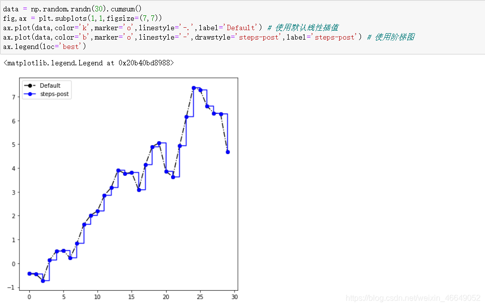
7.1.2 颜色、标记与线类型
matplotlib的主函数plot接受带有x和y的数组以及一些可选的字符串缩写参数来指明颜色和线类型。
颜色由参数color或c指定,有如下选择:
=============    ===============================
character        color
=============    ===============================
``'b'``          blue 蓝
``'g'``          green 绿
``'r'``          red  红
``'c'``          cyan 青
``'m'``          magenta 品红色
``'y'``          yellow 黄
``'k'``          black  黑
``'w'``          white  白
=============    ===============================
标记由参数marker指定,有如下选择:
=============    ===============================
character        description
=============    ===============================
``'.'``          point marker  点标记
``','``          pixel marker
``'o'``          circle marker 圆形标记
``'v'``          triangle_down marker
``'^'``          triangle_up marker
``'<'``          triangle_left marker
``'>'``          triangle_right marker
``'1'``          tri_down marker
``'2'``          tri_up marker
``'3'``          tri_left marker
``'4'``          tri_right marker
``'s'``          square marker
``'p'``          pentagon marker
``'*'``          star marker
``'h'``          hexagon1 marker
``'H'``          hexagon2 marker
``'+'``          plus marker
``'x'``          x marker
``'D'``          diamond marker
``'d'``          thin_diamond marker
``'|'``          vline marker
``'_'``          hline marker
=============    ===============================
标记大小由markersize 或 ms指定
线类型由linestyle 或 ls指定,有如下选择:
=============    ===============================
character        description
=============    ===============================
``'-'``          solid line style  实线
``'--'``         dashed line style  虚线
``'-.'``         dash-dot line style
``':'``          dotted line style
=============    ===============================
线宽度由linewidth 或 lw指定
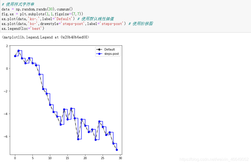
同时也可以使用样式字符串形式。官方文档中是这样定义的:
fmt : str, optional
    A format string, e.g. 'ro' for red circles. See the *Notes*
    section for a full description of the format strings.

    Format strings are just an abbreviation for quickly setting
    basic line properties. All of these and more can also be
    controlled by keyword arguments.

    This argument cannot be passed as keyword.

**Format Strings**

A format string consists of a part for color, marker and line::

    fmt = '[marker][line][color]'

Each of them is optional. If not provided, the value from the style
cycle is used. Exception: If ``line`` is given, but no ``marker``,
the data will be a line without markers.

Other combinations such as ``[color][marker][line]`` are also
supported, but note that their parsing may be ambiguous.
它的大意是:样式字符串不能作为关键字传递,样式字符串的排列方式有[marker][line][color],也可以是[color][marker][line]。
7.1.3刻度、标签、图例
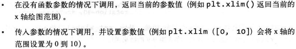
pyplot接口中有xlim方法来控制绘图范围,有xticks方法来控制刻度位置,有xticklabels方法来控制刻度标签,xlabel方法来控制轴标签,title方法来控制标题。我们可以在两种方式中使用。
所有的这些方法都会在当前创建的AxesSubplot上生效。这些方法中每一个对应于子图自身的两个方法。
xlim方法—ax.get_lim与ax.set_lim
xticks方法—ax.get_xticks与ax.set_xticks
xticklabels方法—ax.get_xticklabels与ax.set_xticklabels
xlabel方法—ax.get_xlabel与ax.set_xlabel
title方法—ax.get_title与ax.set_title
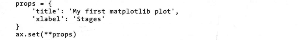
7.1.3.1设置标题、轴标签、刻度和刻度标签
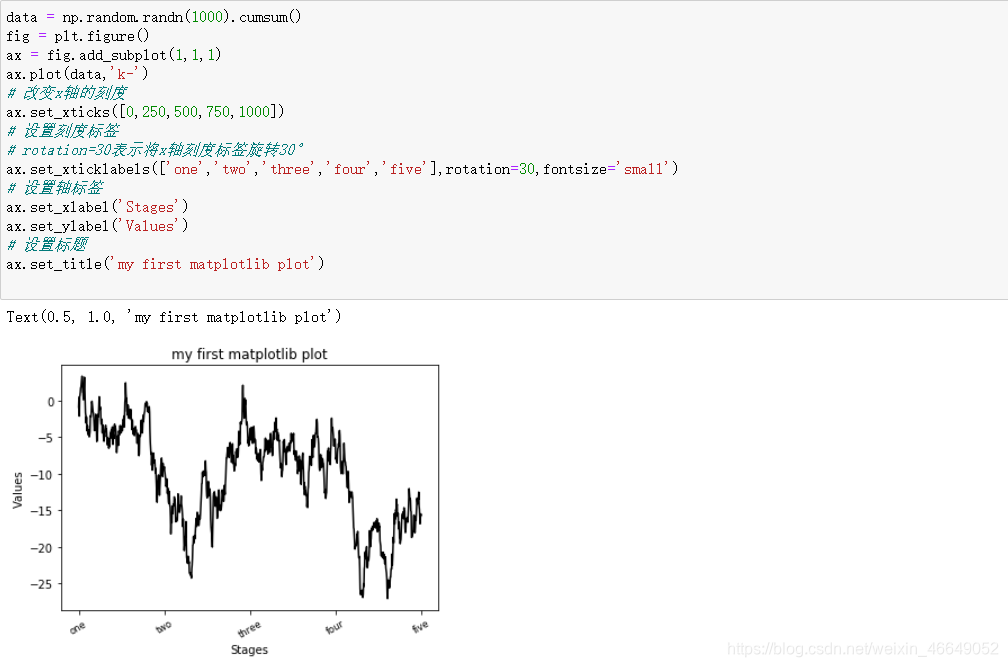
轴的类型拥有一个set方法,允许批量设置绘图属性。
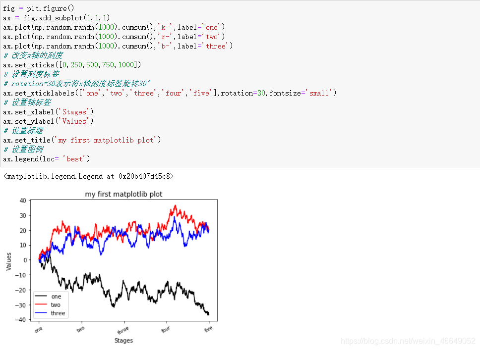
7.1.3.2添加图例
图例是用来区分绘图元素的重要内容。最简单的方式是在plot方法中传入label参数,然后调用plt.legend或者ax.legend方法自动生成图例。其中legend方法中参数loc控制图例的位置。
其中loc参数有如下选择:
loc : str or pair of floats, default: :rc:`legend.loc` ('best' for axes, 'upper right' for figures)
    The location of the legend.

    The strings
    ``'upper left', 'upper right', 'lower left', 'lower right'``
    place the legend at the corresponding corner of the axes/figure.

    The strings
    ``'upper center', 'lower center', 'center left', 'center right'``
    place the legend at the center of the corresponding edge of the
    axes/figure.

    The string ``'center'`` places the legend at the center of the axes/figure.

    The string ``'best'`` places the legend at the location, among the nine
    locations defined so far, with the minimum overlap with other drawn
    artists.  This option can be quite slow for plots with large amounts of
    data; your plotting speed may benefit from providing a specific location.

    The location can also be a 2-tuple giving the coordinates of the lower-left
    corner of the legend in axes coordinates (in which case *bbox_to_anchor*
    will be ignored).

    For back-compatibility, ``'center right'`` (but no other location) can also
    be spelled ``'right'``, and each "string" locations can also be given as a
    numeric value:

        ===============   =============
        Location String   Location Code
        ===============   =============
        'best'            0
        'upper right'     1
        'upper left'      2
        'lower left'      3
        'lower right'     4
        'right'           5
        'center left'     6
        'center right'    7
        'lower center'    8
        'upper center'    9
        'center'          10
        ===============   =============
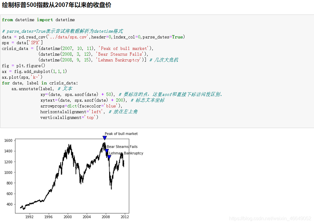
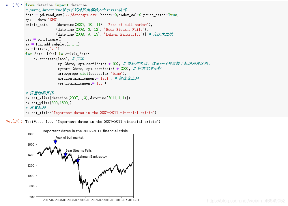
7.1.4注释与子图加工
在图表上绘制注释(可能会包含文本、箭头以及其他图形),可以使用text、arrow和annote方法来添加注释和文本。
通过设置绘图范围,放大某一部分。
Annotate the point *xy* with text *text*.

In the simplest form, the text is placed at *xy*.

Optionally, the text can be displayed in another position *xytext*.
An arrow pointing from the text to the annotated point *xy* can then
be added by defining *arrowprops*.

Parameters
----------
text : str 文本
    The text of the annotation.  *s* is a deprecated synonym for this
    parameter.

xy : (float, float) 标注点的位置
    The point *(x,y)* to annotate.

xytext : (float, float), optional  标注文本位置
    The position *(x,y)* to place the text at.
    If *None*, defaults to *xy*.

xycoords : str, `.Artist`, `.Transform`, callable or tuple, optional

    The coordinate system that *xy* is given in. The following types
    of values are supported:

    - One of the following strings:

      =================   =============================================
      Value               Description
      =================   =============================================
      'figure points'     Points from the lower left of the figure
      'figure pixels'     Pixels from the lower left of the figure
      'figure fraction'   Fraction of figure from lower left
      'axes points'       Points from lower left corner of axes
      'axes pixels'       Pixels from lower left corner of axes
      'axes fraction'     Fraction of axes from lower left
      'data'              Use the coordinate system of the object being
                          annotated (default)
      'polar'             *(theta,r)* if not native 'data' coordinates
      =================   =============================================

    - An `.Artist`: *xy* is interpreted as a fraction of the artists
      `~matplotlib.transforms.Bbox`. E.g. *(0, 0)* would be the lower
      left corner of the bounding box and *(0.5, 1)* would be the
      center top of the bounding box.

    - A `.Transform` to transform *xy* to screen coordinates.

    - A function with one of the following signatures::

        def transform(renderer) -> Bbox
        def transform(renderer) -> Transform

      where *renderer* is a `.RendererBase` subclass.

      The result of the function is interpreted like the `.Artist` and
      `.Transform` cases above.

    - A tuple *(xcoords, ycoords)* specifying separate coordinate
      systems for *x* and *y*. *xcoords* and *ycoords* must each be
      of one of the above described types.

    See :ref:`plotting-guide-annotation` for more details.

    Defaults to 'data'.

textcoords : str, `.Artist`, `.Transform`, callable or tuple, optional
    The coordinate system that *xytext* is given in.

    All *xycoords* values are valid as well as the following
    strings:

    =================   =========================================
    Value               Description
    =================   =========================================
    'offset points'     Offset (in points) from the *xy* value
    'offset pixels'     Offset (in pixels) from the *xy* value
    =================   =========================================

    Defaults to the value of *xycoords*, i.e. use the same coordinate
    system for annotation point and text position.

arrowprops : dict, optional
    The properties used to draw a
    `~matplotlib.patches.FancyArrowPatch` arrow between the
    positions *xy* and *xytext*.

    If *arrowprops* does not contain the key 'arrowstyle' the
    allowed keys are:

    ==========   ======================================================
    Key          Description
    ==========   ======================================================
    width        The width of the arrow in points
    headwidth    The width of the base of the arrow head in points
    headlength   The length of the arrow head in points
    shrink       Fraction of total length to shrink from both ends
    ?            Any key to :class:`matplotlib.patches.FancyArrowPatch`
    ==========   ======================================================

    If *arrowprops* contains the key 'arrowstyle' the
    above keys are forbidden.  The allowed values of
    ``'arrowstyle'`` are:

    ============   =============================================
    Name           Attrs
    ============   =============================================
    ``'-'``        None
    ``'->'``       head_length=0.4,head_width=0.2
    ``'-['``       widthB=1.0,lengthB=0.2,angleB=None
    ``'|-|'``      widthA=1.0,widthB=1.0
    ``'-|>'``      head_length=0.4,head_width=0.2
    ``'<-'``       head_length=0.4,head_width=0.2
    ``'<->'``      head_length=0.4,head_width=0.2
    ``'<|-'``      head_length=0.4,head_width=0.2
    ``'<|-|>'``    head_length=0.4,head_width=0.2
    ``'fancy'``    head_length=0.4,head_width=0.4,tail_width=0.4
    ``'simple'``   head_length=0.5,head_width=0.5,tail_width=0.2
    ``'wedge'``    tail_width=0.3,shrink_factor=0.5
    ============   =============================================

    Valid keys for `~matplotlib.patches.FancyArrowPatch` are:

    ===============  ==================================================
    Key              Description
    ===============  ==================================================
    arrowstyle       the arrow style
    connectionstyle  the connection style
    relpos           default is (0.5, 0.5)
    patchA           default is bounding box of the text
    patchB           default is None
    shrinkA          default is 2 points
    shrinkB          default is 2 points
    mutation_scale   default is text size (in points)
    mutation_aspect  default is 1.
    ?                any key for :class:`matplotlib.patches.PathPatch`
    ===============  ==================================================

    Defaults to None, i.e. no arrow is drawn.

annotation_clip : bool or None, optional
    Whether to draw the annotation when the annotation point *xy* is
    outside the axes area.

    - If *True*, the annotation will only be drawn when *xy* is
      within the axes.
    - If *False*, the annotation will always be drawn.
    - If *None*, the annotation will only be drawn when *xy* is
      within the axes and *xycoords* is 'data'.

    Defaults to *None*.

**kwargs
    Additional kwargs are passed to `~matplotlib.text.Text`.

Returns
-------
annotation : `.Annotation`

See Also
--------
:ref:`plotting-guide-annotation`.
matplotlib中含有多种常见图形的对象,这些对象的引用是patches。图形的全集位于matplotlib.patches。在图表中添加图形时,需要生成patch对象,并调用ax.add_patch()将对象加入到子图中。

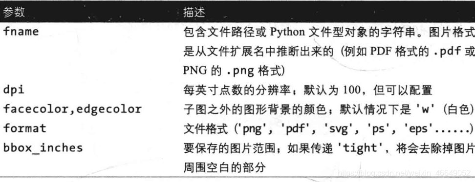
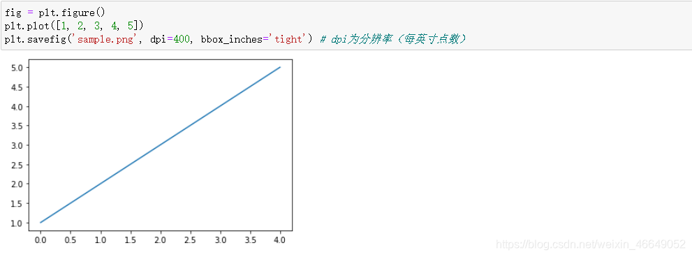
7.1.5将图片保存到文件中
使用plt.savefig将图片保存到文件中,该方法有如下参数:
7.1.6matplotlib设置
用于全局设置包括图形大小,子图间距,颜色,字体大小,网格样式等,常使用rc方法
Set the current rc params.  *group* is the grouping for the rc, e.g.,
for ``lines.linewidth`` the group is ``lines``, for
``axes.facecolor``, the group is ``axes``, and so on.  Group may
also be a list or tuple of group names, e.g., (*xtick*, *ytick*).
*kwargs* is a dictionary attribute name/value pairs, e.g.,::

  rc('lines', linewidth=2, color='r')

sets the current rc params and is equivalent to::

  rcParams['lines.linewidth'] = 2
  rcParams['lines.color'] = 'r'

The following aliases are available to save typing for interactive
users:

=====   =================
Alias   Property
=====   =================
'lw'    'linewidth'
'ls'    'linestyle'
'c'     'color'
'fc'    'facecolor'
'ec'    'edgecolor'
'mew'   'markeredgewidth'
'aa'    'antialiased'
=====   =================

Thus you could abbreviate the above rc command as::

      rc('lines', lw=2, c='r')


Note you can use python's kwargs dictionary facility to store
dictionaries of default parameters.  e.g., you can customize the
font rc as follows::

  font = {

    'family' : 'monospace',
          'weight' : 'bold',
          'size'   : 'larger'}

  rc('font', **font)  # pass in the font dict as kwargs

This enables you to easily switch between several configurations.  Use
``matplotlib.style.use('default')`` or :func:`~matplotlib.rcdefaults` to
restore the default rc params after changes.
7.2 使用pandas与seaborn绘图
seaborn简化了常用可视化类型的生成。导入seaborn会修改默认的matplotlib配色方案和绘图样式,这会提高图表的可读性与美观性。即使不使用seaborn的API,导入seaborn也可以为matplotlib图表提供更好的视觉美观度。
7.2.1折线图
Series和DataFrame都有plot属性,用于绘制基本图形。默认情况下,绘制的是折线图。Series对象的索引传入matplotlib作为绘图的x轴,可以通过传入use_index = False来禁用该功能。
Series.plot参数:


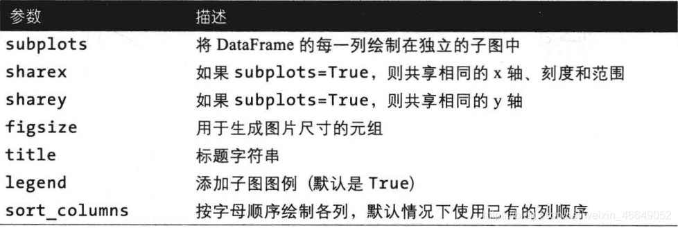
DataFrame的plot方法在同一个子图中将每一列绘制为不同的折线,并自动生成图例。
DataFrame.plot参数:

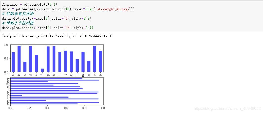
7.2.2柱状图(垂直或水平)
plot.bar()和plot.barh()可以绘制垂直和水平柱状图。在绘制柱状图时,Series或DataFrame的索引将会被用作x轴刻度(bar)或y轴刻度(barh)。
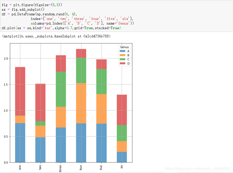
DataFrame中,柱状图将每一行中的值分组到并排的柱子中的一组。

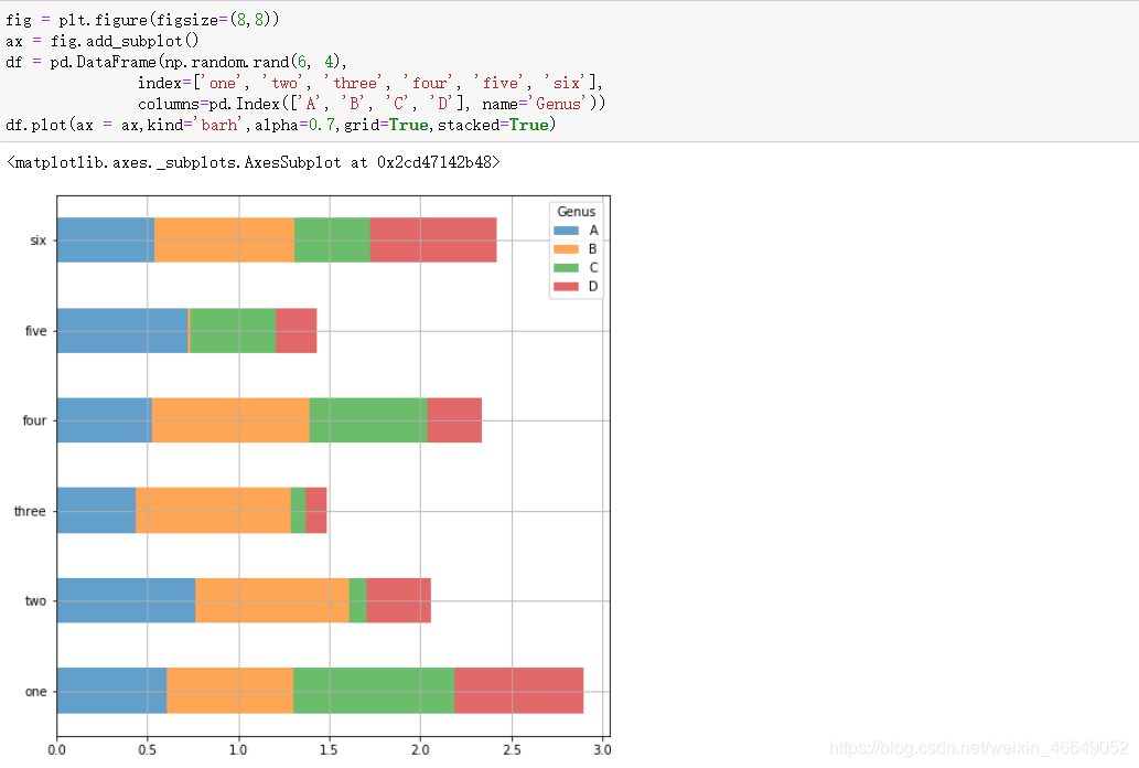
我们可以设置stacked=True来生成堆积柱状图,会使得每一行的值堆积在一起。
堆积垂直柱状图:
堆积水平柱状图:
使用s.value_counts().plot.bar()可以有效地对Series值频率进行可视化
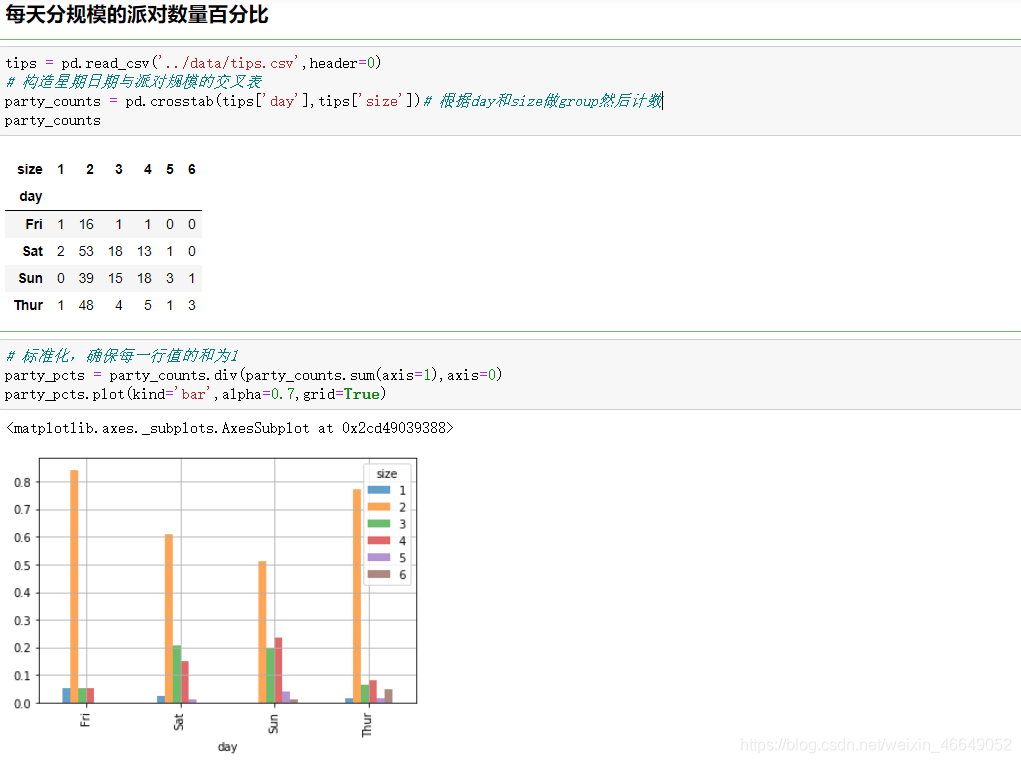
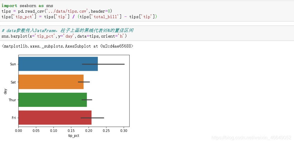
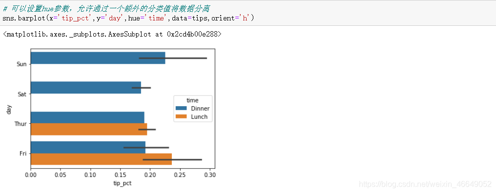
对于在绘图前需要聚合或汇总的数据,使用seaborn包会使工作简单。
绘制小费占总消费的百分比:
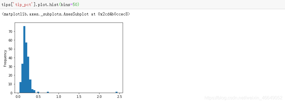
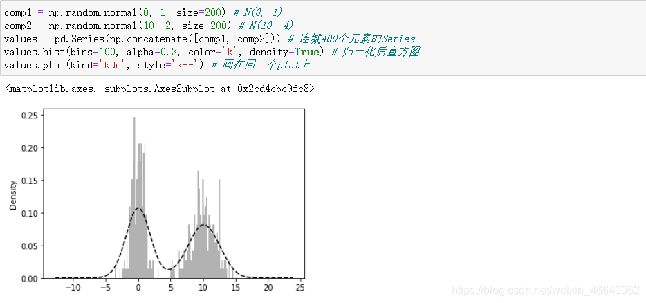
7.2.3直方图和密度图
直方图是一种条形图,用于给出值频率的离散显示。数据点被分成离散的,均匀间隔的箱,并且绘制每个箱中数据点的数量。
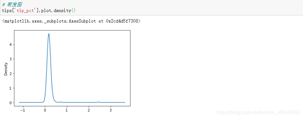
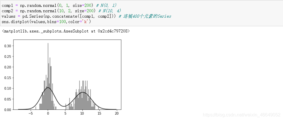
密度图是一种与直方图相关的图表类型,它通过计算可能产生观测数据的连续概率分布估计而产生。通常做法是将这种分布近似为‘内核’的混合。
seaborn中displot方法可以绘制直方图与连续密度估计
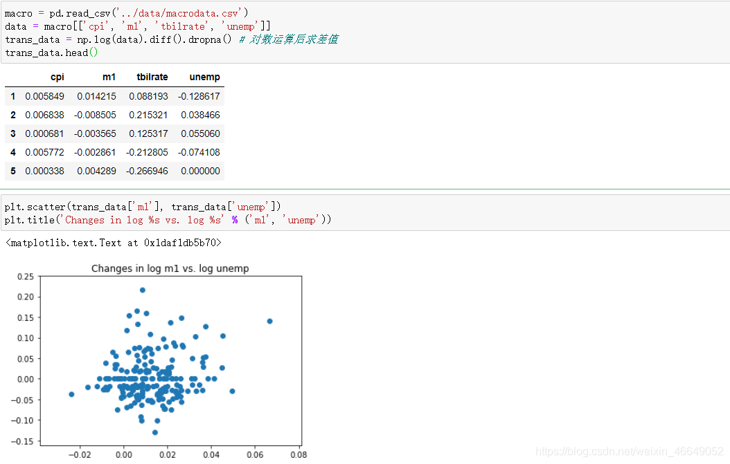
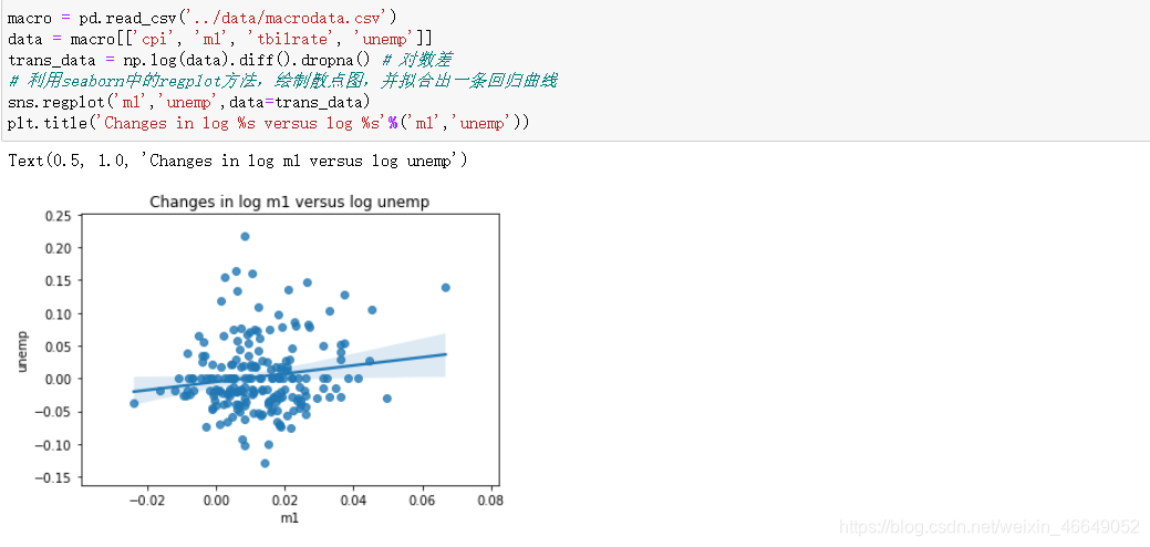
7.2.4散点图与点图
散点图或者点图是用于检验两个一维数据序列之间的关系。
利用seaborn中的regplot方法,绘制散点图,并拟合出一条回归曲线
画散点矩阵图
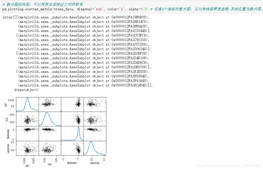
seaborn中有一个pairplot函数,它支持在对角线上放置每个变量的散点图或者密度估计图。其中参数plot_ksw,这个参数是我们能够将配置选项传递给非对角线元素上的各个元素的调用。
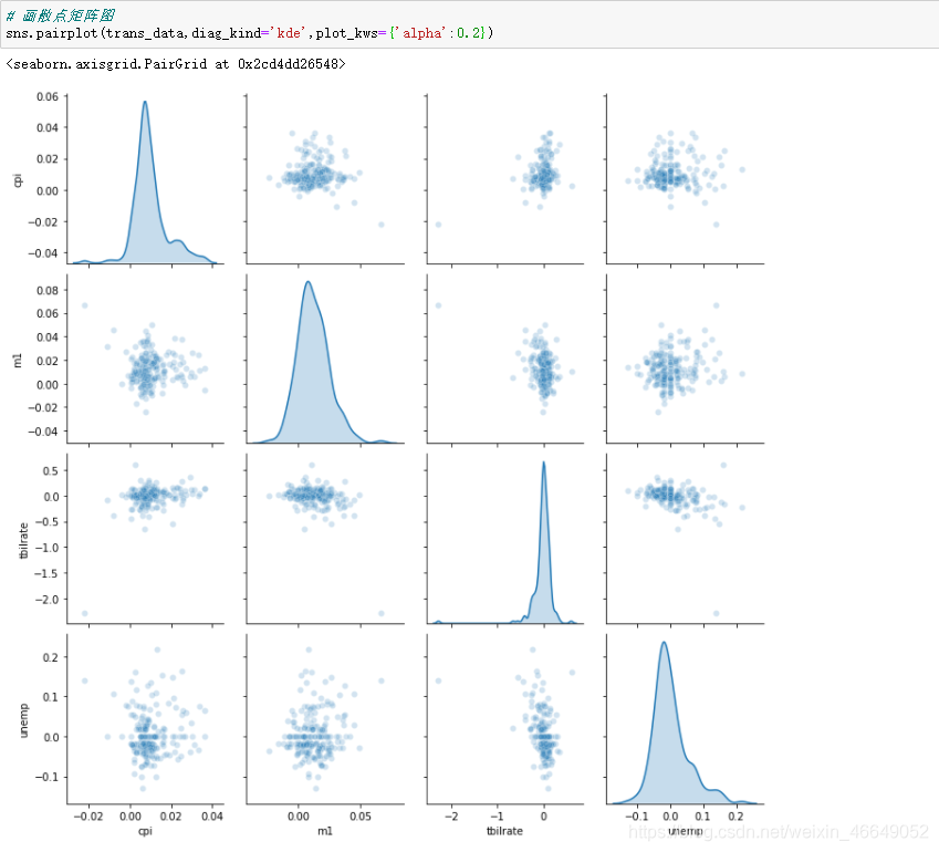
与matplotlib中相比,是不是显得磅礴大气呢?
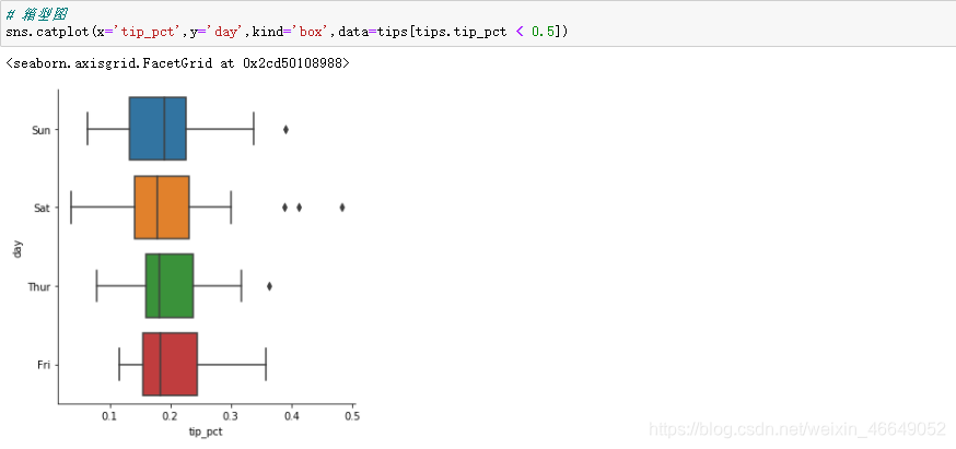
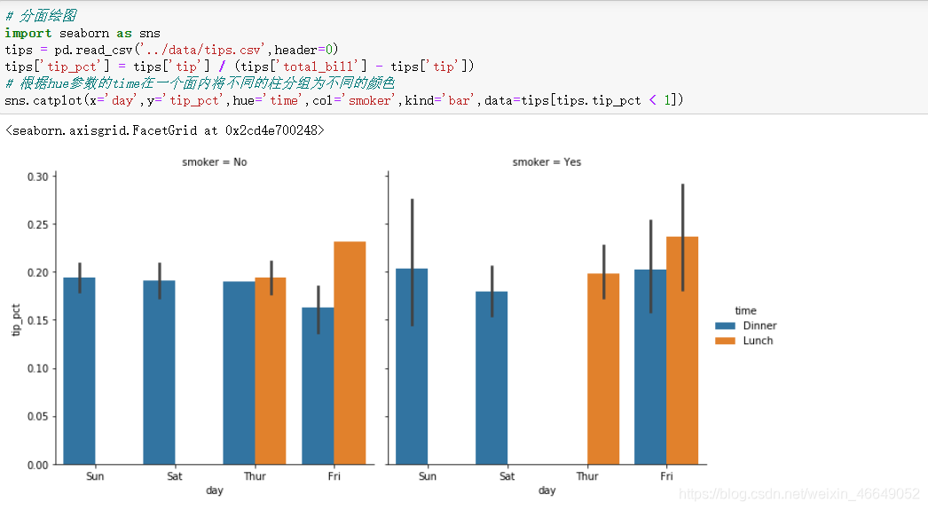
7.2.5分面网格和分类数据
使用分面网格是利用多种分组变量对数据进行可视化的方式。seaborn中有一个函数catplot,它可以简化多种分面绘图。
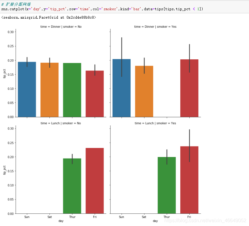
catplot还支持其他图类型,具体取决于要显示的内容。例如:箱形图