机器学习笔记 - 前馈神经网络(FFNN)用作回归问题的波士顿房价预测

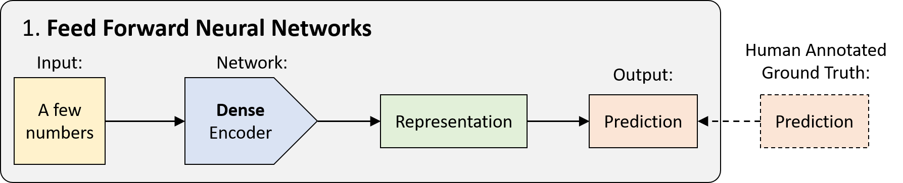
FFNN的历史可以追溯到1940年代，它是没有任何循环的网络。数据从输入到输出通过一次传递，而没有以前的任何“状态存储”。 从技术上讲，深度学习中的大多数网络都可以被认为是FFNN，但通常“ FFNN”是指其最简单的变体：紧密连接的多层感知器（MLP）。

深度前馈网络（通常也称为前馈神经网络）或多层感知器（MLP）是典型的深度学习模型。前馈网络的目标是近似某个函数f *。 例如，对于分类器，y = f *（x）将输入x映射到类别y。 前馈网络定义映射y = f（x;θ）并学习参数θ的值，以得到最佳的函数逼近。

参考代码

# 波士顿房价预测

# TensorFlow and tf.keras
import tensorflow as tf
from tensorflow import keras
from tensorflow.keras.layers import Conv2D, MaxPooling2D, Dropout, Flatten, Dense

# Commonly used modules 常用模块
import numpy as np
import os
import sys

# Images, plots, display, and visualization
import matplotlib.pyplot as plt
import pandas as pd
import seaborn as sns
import cv2
import IPython
from six.moves import urllib


# 获取数据集
# 也可以自行下载 https://storage.googleapis.com/tensorflow/tf-keras-datasets/boston_housing.npz
(train_features, train_labels), (test_features, test_labels) = keras.datasets.boston_housing.load_data()

# get per-feature statistics (mean, standard deviation) from the training set to normalize by
# 从训练集中获取每个特征的统计信息（均值，标准差）
train_mean = np.mean(train_features, axis=0)
train_std = np.std(train_features, axis=0)
train_features = (train_features - train_mean) / train_std

# 构建模型
def build_model():
    model = keras.Sequential([
        Dense(20, activation=tf.nn.relu, input_shape=[len(train_features[0])]),
        Dense(1)
    ])

    model.compile(optimizer=tf.optimizers.Adam(), loss='mse', metrics=['mae', 'mse'])
    return model


# this helps makes our output less verbose but still shows progress
class PrintDot(keras.callbacks.Callback):
    def on_epoch_end(self, epoch, logs):
        if epoch % 100 == 0: print('')
        print('.', end='')

# 构建模型
model = build_model()
# 当监测数量停止改善时停止训练
early_stop = keras.callbacks.EarlyStopping(monitor='val_loss', patience=50)
# 训练模型
history = model.fit(train_features, train_labels, epochs=1000, verbose=0, validation_split = 0.1,
                    callbacks=[early_stop, PrintDot()])
# 创建一个DataFrame
hist = pd.DataFrame(history.history)
hist['epoch'] = history.epoch

# show RMSE measure to compare to Kaggle leaderboard on https://www.kaggle.com/c/boston-housing/leaderboard
rmse_final = np.sqrt(float(hist['val_mse'].tail(1)))
print()
print('Final Root Mean Square Error on validation set: {}'.format(round(rmse_final, 3)))


# 让我们在训练和验证集上绘制损失函数度量。
def plot_history():
    plt.figure()
    plt.xlabel('Epoch')
    plt.ylabel('Mean Square Error [Thousand Dollars$^2$]')
    plt.plot(hist['epoch'], hist['mse'], label='Train Error')
    plt.plot(hist['epoch'], hist['val_mse'], label = 'Val Error')
    plt.legend()
    plt.ylim([0,50])

plot_history()


#接下来，比较模型在测试数据集上的表现：
test_features_norm = (test_features - train_mean) / train_std
mse, _, _ = model.evaluate(test_features_norm, test_labels)
rmse = np.sqrt(mse)
print('Root Mean Square Error on test set: {}'.format(round(rmse, 3)))