前言
此篇文章是接上一篇内容的,上一篇的传送门:
在上一篇中,我们详细debug了yolov3源码models.py文件,并重点介绍了模型创建的部分。models.py里面除了Darknet类之外,还有一个重要的类YOLOLayer,它涉及了anchor的操作、GT和Pred值的放缩、iou的计算以及loss的重要内容。基本上搞懂了这个类,那么yolov3的代码核心就明白了50%以上,对于yolov3这个项目来讲,这也是最难懂的一部分代码。
希望大家再接再厉,跟着我一起debug这一部分代码,首先大家先思考下下面几个核心问题,并且带着问题来一起研究:
- anchor和gt怎么一一对应?
- anchor和inference怎么一一对应?
- yolov3怎么判断正样本负样本?
- yolov3的loss是怎么计算的?
在进入代码debug前,我们先通过一张图回顾下yolov3的结构:
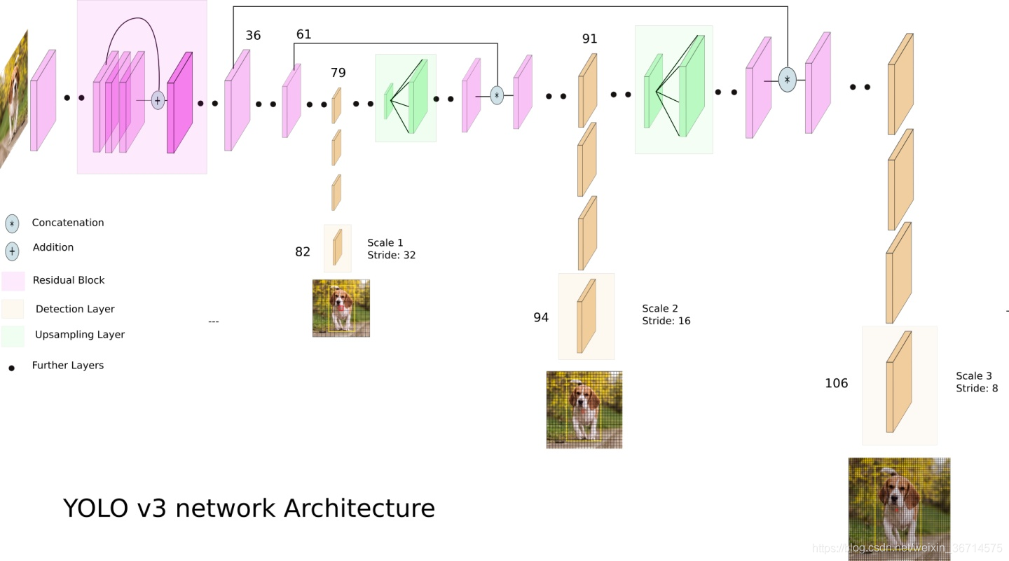
这张图清晰的描述了yolov3的网络架构:图片送入darknet53 backbone然后在经过几个卷积,在第79层产生分支,一路继续卷积在第82层获得第一个yolo 输出(stride=32),另一路则经过2倍上采样与第61层的feature map进行融合(concat),按照这种分支结构,分别产生了3个yolo 输出。分别为下采样32倍、16倍和8倍,对应的resolution从小到大。这里问大家一个问题,32倍下采样的输出(对应小resolution)和8倍下采样的输出(对应大resolution),哪个更擅长预测小物体?
答案是小resolution适合预测大物体,而大resolution适合小物体。这里容易有个误区就小resolution对应的感受野大,可能会误认为是预测达大物体。其实这个问题可以这样思考,下采样过多,那么在原图尺寸上的小物体可能就会丢失了信息,难以恢复。所以对于小物体的预测,增大预测图的resolution是个靠谱的思路。在目标检测和语义分割的很多研究中都沿用了这种思路。
好了,下面我们开始正式分析YOLOLayer的源码。
Part2. models.py里面的YOLOLayer源码分析
YOLOLayer源码分析会重点涉及到以下的一些函数,所以debug前我们先对以下函数打上断点:
- YOLOLayer里的forward()
- models.py文件里的compute_grid_offsets()
- utils.py文件里的build_targets()、bbox_wh_iou()、bbox_iou()
下面我们先从YOLOLayer里开始,先看下__init__()函数源码:
    def __init__(self, anchors, num_classes, img_dim=416):
        super(YOLOLayer, self).__init__()
        self.anchors = anchors
        self.num_anchors = len(anchors)
        self.num_classes = num_classes
        self.ignore_thres = 0.5
        self.mse_loss = nn.MSELoss()
        self.bce_loss = nn.BCELoss()
        self.obj_scale = 1
        self.noobj_scale = 100
        self.metrics = {

    }
        self.img_dim = img_dim
        self.grid_size = 0  # grid size
这里初始化了一些参数,后面用到的时候我们再分析,重点看下forward()函数:
    def forward(self, x, targets=None, img_dim=None):
        """
        :param x: B C H W 比如[2 255 13 13]
        :param targets:  B 6
        :param img_dim:
        :return:
        """

        # Tensors for cuda support
        FloatTensor = torch.cuda.FloatTensor if x.is_cuda else torch.FloatTensor
        LongTensor = torch.cuda.LongTensor if x.is_cuda else torch.LongTensor

        self.img_dim = img_dim #default 416
        num_samples = x.size(0)
        grid_size = x.size(2)  #13 26 52
这里只需明确下输入的x的维度是[B C H W],我们都以32倍下采样的输出图为例,来剖析YOLOLayer,debug我只用了1张图片,所以我的x的shape是[1,3, 13, 13],num_samples对应的就是1,而grid_size对应的是13(其他yolo layer则相应对应26, 52)。
    # B A H W X 比如[2 3 13 13 85] 85=80 + 5
        prediction = (
            x.view(num_samples, self.num_anchors, self.num_classes + 5, grid_size, grid_size)
            .permute(0, 1, 3, 4, 2)  # class/localization 数值放到最后一维 方便进行sigmoid
            .contiguous()  # 调用permute/transpose之后 再调用view需要率先调用contigious
        )

        # Get outputs
        x = torch.sigmoid(prediction[..., 0])  # Center x  #B A H W
        y = torch.sigmoid(prediction[..., 1])  # Center y  #B A H W
        w = prediction[..., 2]  # Width                    #B A H W
        h = prediction[..., 3]  # Height                   #B A H W
        pred_conf = torch.sigmoid(prediction[..., 4])  # Conf
        pred_cls = torch.sigmoid(prediction[..., 5:])  # Cls pred.
x对应正向传播的输出,所以通过permute()函数调整通道顺序为[B ,A ,C+5, H, W],其中B是BatchSize,我们选取为1,A是Anchor数量,默认采用3个Anchor所以A=3,C是class数量,5是一个confidence score+4个boundingbox坐标位置xywh,H,W是输出特征图的grid size,这里是13。最后我们通过sigmoid对这些输出值分别进行激活,值域全部处于(0,1)区间。
这里需要注意的是x,y,w,h全部是以grid网格(比如13x13)坐标为基准的相对值。x,y是boundingbox的中心点,以grid网格的左上角为参照。w,h也是以grid为单位长度的相对值。也就是所有的localization的计算我们都是在grid层面上进行的,而不是原图上面进行的。
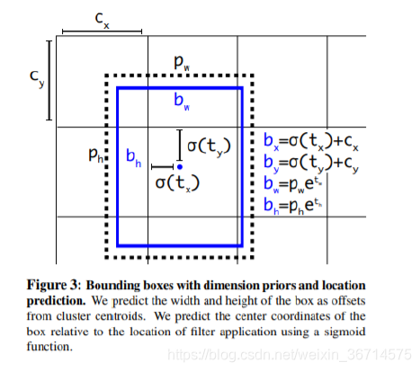
现在大家再观察论文中的这张图是不是就完全对应上了呢?
        if grid_size != self.grid_size:
            self.compute_grid_offsets(grid_size, cuda=x.is_cuda)
这两句主要是看compute_grid_offsets()这个函数:
    def compute_grid_offsets(self, grid_size, cuda=True):
        self.grid_size = grid_size
        g = self.grid_size
        FloatTensor = torch.cuda.FloatTensor if cuda else torch.FloatTensor
        self.stride = self.img_dim / self.grid_size  #格点大小
        # Calculate offsets for each grid
        self.grid_x = torch.arange(g).repeat(g, 1).view([1, 1, g, g]).type(FloatTensor)  # gxg
        self.grid_y = torch.arange(g).repeat(g, 1).t().view([1, 1, g, g]).type(FloatTensor) # (gxg)T
        # 把anchor放缩到grid上  scaled_anchors [3,2]
        self.scaled_anchors = FloatTensor([(a_w / self.stride, a_h / self.stride) for a_w, a_h in self.anchors])
        self.anchor_w = self.scaled_anchors[:, 0:1].view((1, self.num_anchors, 1, 1))   #scaled w  [1,3,1,1]
        self.anchor_h = self.scaled_anchors[:, 1:2].view((1, self.num_anchors, 1, 1))   #scaled h  [1,3,1,1]
self.grid_x和self.grid_y这两个变量其实就是保存了grid中每个点的坐标。self.scaled_anchors()是对于anchor的数值除以stride,换句话说就是把anchor的长宽也变换到了gird网格的相对值。self.anchor_w和self.anchor_h进一步拿到了每个anchor的相对长宽。所以GT、anchor、pred都是相对值,对应的iou的计算也是在网格层面进行计算的。
   # Add offset and scale with anchors  都是用gird来表示的 而不是原始数值
        pred_boxes = FloatTensor(prediction[..., :4].shape)  # B A H W 4
        pred_boxes[..., 0] = x.data + self.grid_x
        pred_boxes[..., 1] = y.data + self.grid_y
        pred_boxes[..., 2] = torch.exp(w.data) * self.anchor_w
        pred_boxes[..., 3] = torch.exp(h.data) * self.anchor_h

        output = torch.cat(
            (
                pred_boxes.view(num_samples, -1, 4) * self.stride,
                pred_conf.view(num_samples, -1, 1),
                pred_cls.view(num_samples, -1, self.num_classes),
            ),
            -1,
        )
这几行就是在计算上图中的bx,by,bw,bh。标记一下几个变量的shape:
| 变量名 | shape |
|---|---|
| x | [B A H W] |
| y | [B A H W] |
| grid_x | [1 1 H W] |
| grid_y | [1 1 H W] |
| w | [B A H W] |
| h | [B A H W] |
| anchor_w | [1 A 1 1] |
| anchor_w | [1 A 1 1] |
这样是不是就清晰了?tensor是如何进行计算的。
output输出的时候需要乘以stride,来恢复到原图上的尺寸。同时通过view()将A*H*W被挤进了一个维度,可以理解为把所有网格上所有anchor产生的输出都排列起来,形成了[B, A*H*W, …]的输出,torch,cat()在最后一个维度上将这些结果拼接,最终得到了output 的维度就是[B,A*H*W,4+1+C],而且这时候output里面的的localization信息已经通过乘以stride恢复到原图尺寸了。
以上就是处理inference的数值流程。但是我们在计算loss的时候并不需要恢复到原图尺寸,这里只是为了输出。下面我们会遇到一个重要的函数,build_targets()用于处理GT的信息。
        if targets is None:
            return output, 0
        else:
            iou_scores, class_mask, obj_mask, noobj_mask, tx, ty, tw, th, tcls, tconf = build_targets(
                pred_boxes=pred_boxes, #  [B A H W 4]  grid为单位的相对值
                pred_cls=pred_cls,   #   [B A H W 80]
                target=targets,   # B*T 6   target原始文件里类似 [0 0.515 0.5 0.21694873 0.18286777] 通过collate_fn()增加sample_index维度
                anchors=self.scaled_anchors,  # [3, 2]
                ignore_thres=self.ignore_thres,
            )
这个函数有很多输入输出,我们先看输入的维度吧:
| 输入 | 维度 |
|---|---|
| pred_boxes | [B A H W 4] |
| pred_cls | [B A H W 80] |
| targets | [T 6] |
| anchors | [A 2] |
其中pred_boxes是网格单位的相对值,targets中的T是Σti * bi,也就是所有batch内的target数量之和。我们在build_targets()函数增加断点,进一步debug:
def build_targets(pred_boxes, pred_cls, target, anchors, ignore_thres):
    """
        1.通过target的中心点判断标记哪个grid负责预测target
        计算每个grid的3个anchor与target的iou, 标记哪些anchor是正样本 哪些是负样本
    :param pred_boxes:  [B A H W 4]  grid为单位的相对值
    :param pred_cls:  [B A H W 80]
    :param target: [T ,6]    6代表:index, class, x_center, y_center, w, h
            target原始文件里类似 [0 0.515 0.5 0.21694873 0.18286777] 是针对原图的比例 通过collate_fn()增加sample_index维度
    :param anchors: [3, 2]  scaled
    :param ignore_thres:
    :return:
    """

    BoolTensor = torch.cuda.BoolTensor if pred_boxes.is_cuda else torch.BoolTensor
    FloatTensor = torch.cuda.FloatTensor if pred_boxes.is_cuda else torch.FloatTensor
    # pred_boxes B A H W 4
    nB = pred_boxes.size(0)
    nA = pred_boxes.size(1)
    nC = pred_cls.size(-1)
    nG = pred_boxes.size(2)

    # Output tensors
    obj_mask = BoolTensor(nB, nA, nG, nG).fill_(0)  # [B A G G]  G:13, 26, 52...  布尔值
    noobj_mask = BoolTensor(nB, nA, nG, nG).fill_(1) # [B A G G]  G:13, 26, 52...  布尔值
    class_mask = FloatTensor(nB, nA, nG, nG).fill_(0) # [B A G G]  G:13, 26, 52...  float
    iou_scores = FloatTensor(nB, nA, nG, nG).fill_(0) # [B A G G]  G:13, 26, 52...  float
    tx = FloatTensor(nB, nA, nG, nG).fill_(0) # [B A G G]  G:13, 26, 52...  float
    ty = FloatTensor(nB, nA, nG, nG).fill_(0) # [B A G G]  G:13, 26, 52...  float
    tw = FloatTensor(nB, nA, nG, nG).fill_(0) # [B A G G]  G:13, 26, 52...  float
    th = FloatTensor(nB, nA, nG, nG).fill_(0) # [B A G G]  G:13, 26, 52...  float
    tcls = FloatTensor(nB, nA, nG, nG, nC).fill_(0) # [B A G G C]  G:13, 26, 52...  float

    # Convert to position relative to box
    target_boxes = target[:, 2:6] * nG  #从针对原图的比例转换为针对格点的比例  x_center, y_center, h, w
    gxy = target_boxes[:, :2]  # T 2  grid level
    gwh = target_boxes[:, 2:]  # T 2  grid level
    # Get anchors with best iou
    # 这里传入的都是相对格点的数值
    ious = torch.stack([bbox_wh_iou(anchor, gwh) for anchor in anchors]) # [A, T] A代表anchor T代表与所有target的iou
    best_ious, best_n = ious.max(0)  # best_ious 最大的iou  best_n最大iou对应的anchor编号
    # Separate target values
    b, target_labels = target[:, :2].long().t() # b是sample index  target_labels是标签
    gx, gy = gxy.t()
    gw, gh = gwh.t()
    gi, gj = gxy.long().t()  # .long()相当于向下取整, target 中心点(x,y)落在的格点位置,标记了哪个格点有target
    # Set masks
    # 这里可以这样理解:需要做的是把所有target定位到grid上面,定位每个点需要四个坐标
    # [sample编号b(对应batchsize B), anchor编号(best_n 对应anchors A), grid坐标 x,y] 所以先对每个anchor求b, best_n,
    # 相对偏移量gj gi ,这样把四个坐标放进obj_mask就可以了。这四个坐标长度都是T的索引
    obj_mask[b, best_n, gj, gi] = 1 # B A H W 中标记命中target的位置(有前景)  标记正样本位置
    noobj_mask[b, best_n, gj, gi] = 0 # B A H W 有前景的标为0 其余的就是背景 标为1

    # Set noobj mask to zero where iou exceeds ignore threshold
    # 负样本iou超过阈值的部分不再标记为负样本,也就是这部分不参与loss计算
    for i, anchor_ious in enumerate(ious.t()):   #ious.t()  [T A]  每行代表每个target与A个anchor的iou
        noobj_mask[b[i], anchor_ious > ignore_thres, gj[i], gi[i]] = 0

    # Coordinates  相对值 可以直接做loss回归的
    tx[b, best_n, gj, gi] = gx - gx.floor() #gt 相对于左上角格点的水平偏移量  [B A G G]
    ty[b, best_n, gj, gi] = gy - gy.floor() #gt 相对于左上角格点的垂直偏移量  [B A G G]
    # Width and height
    tw[b, best_n, gj, gi] = torch.log(gw / anchors[best_n][:, 0] + 1e-16) # target相对于对应的anchor的比例 [B A G G]
    th[b, best_n, gj, gi] = torch.log(gh / anchors[best_n][:, 1] + 1e-16) # [B A G G]
    # One-hot encoding of label
    tcls[b, best_n, gj, gi, target_labels] = 1
    # Compute label correctness and iou at best anchor
    class_mask[b, best_n, gj, gi] = (pred_cls[b, best_n, gj, gi].argmax(-1) == target_labels).float()
    iou_scores[b, best_n, gj, gi] = bbox_iou(pred_boxes[b, best_n, gj, gi], target_boxes, x1y1x2y2=False)

    tconf = obj_mask.float()
    return iou_scores, class_mask, obj_mask, noobj_mask, tx, ty, tw, th, tcls, tconf
大部分的tensor shape我已经标注到了代码里,这里有个要提一下的是,target的shape是[T 6],T是Batch内全部的target数量,6是sample_index, class, x_center, y_center, H, W。sample_index是DataSet构建里collate_fn()的结果,增加了一个维度,代表这个target来自于batch里的哪个样本。
    # Output tensors
    obj_mask = BoolTensor(nB, nA, nG, nG).fill_(0)  # [B A G G]  G:13, 26, 52...  布尔值
    noobj_mask = BoolTensor(nB, nA, nG, nG).fill_(1) # [B A G G]  G:13, 26, 52...  布尔值
    class_mask = FloatTensor(nB, nA, nG, nG).fill_(0) # [B A G G]  G:13, 26, 52...  float
    iou_scores = FloatTensor(nB, nA, nG, nG).fill_(0) # [B A G G]  G:13, 26, 52...  float
    tx = FloatTensor(nB, nA, nG, nG).fill_(0) # [B A G G]  G:13, 26, 52...  float
    ty = FloatTensor(nB, nA, nG, nG).fill_(0) # [B A G G]  G:13, 26, 52...  float
    tw = FloatTensor(nB, nA, nG, nG).fill_(0) # [B A G G]  G:13, 26, 52...  float
    th = FloatTensor(nB, nA, nG, nG).fill_(0) # [B A G G]  G:13, 26, 52...  float
    tcls = FloatTensor(nB, nA, nG, nG, nC).fill_(0) # [B A G G C]  G:13, 26, 52...  float
这里就是产生了一堆mask和索引,后面会用到。
    # Convert to position relative to box
    target_boxes = target[:, 2:6] * nG  #从针对原图的比例转换为针对格点的比例  x_center, y_center, h, w
    gxy = target_boxes[:, :2]  # T 2  grid level
    gwh = target_boxes[:, 2:]  # T 2  grid level
target传入时候是根据原图的比例进行计算的相对值,这里*nG就是放缩到了网格的单位。gxy是前两维度x_center,y_center;gwh是后两维,代表h,w。
ious = torch.stack([bbox_wh_iou(anchor, gwh) for anchor in anchors]) # [A, T] A代表anchor T代表与所有target的iou
这里涉及到新的函数bbox_wh_iou(),打上断点,看下这个函数:
def bbox_wh_iou(wh1, wh2):
    """
        用于scaled target和scaled anchor 进行IOU计算
        每个scaled anchor分别与所有的scaled target做iou计算
        计算iou与中心点无关,只需要计算w,h
    :param wh1: scaled anchor size
    :param wh2: scaled target WH : [T 2]
    :return: 所有target与某个anchor的iou  T
    """
    wh2 = wh2.t()  #[2 T]
    w1, h1 = wh1[0], wh1[1] # W H
    w2, h2 = wh2[0], wh2[1]
    inter_area = torch.min(w1, w2) * torch.min(h1, h2)
    union_area = (w1 * h1 + 1e-16) + w2 * h2 - inter_area
    return inter_area / union_area
输入wh1是scaled anchor,wh2是scaled target。函数里的计算都是element-wise的,所以最后输出的就是T个值。分别代表了所有T个target与anchor的iou数值。
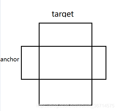
大家可以从上图看到,只要target与anchor有交集,那么他们之间计算iou是不需要中心点坐标的。
ious = torch.stack([bbox_wh_iou(anchor, gwh) for anchor in anchors]) # [A, T] A代表anchor T代表与所有target的iou
那么这里分别计算3个anchor与所有target的iou,最后再stack起来,得到的结果就是[3 T]。
best_ious, best_n = ious.max(0) # best_ious 最大的iou best_n最大iou对应的anchor编号
这里对第0个维度取最大值,实际上就是得到了每个target最大iou的anchor编号,以及iou的数值。
# Separate target values
    b, target_labels = target[:, :2].long().t() # b是sample index  target_labels是标签
    gx, gy = gxy.t()
    gw, gh = gwh.t()
    gi, gj = gxy.long().t()  # .long()相当于向下取整, target 中心点(x,y)落在的格点位置,标记了哪个格点有target
这里拿出了target中的b和class,b代表的就是sample_index,target_labels代表的就是class。
gi, gj = gxy.long().t()
这句是对gxy的坐标进行了向下取整,那么得到的就是左上角的格点坐标。这里实际上就是标记了target所对应的pred值的格点坐标,或者理解为标记哪个格点是前景。将target与inference值一一对应了起来。
    # Set masks
    # 这里可以这样理解:需要做的是把所有target定位到grid上面,定位每个点需要四个坐标
    # [sample编号b(对应batchsize B), anchor编号(best_n 对应anchors A), grid坐标 x,y] 所以先对每个anchor求b, best_n,
    # 相对偏移量gj gi ,这样把四个坐标放进obj_mask就可以了。这四个坐标长度都是T的索引
    obj_mask[b, best_n, gj, gi] = 1 # B A H W 中标记命中target的位置(有前景)  标记正样本位置
    noobj_mask[b, best_n, gj, gi] = 0 # B A H W 有前景的标为0 其余的就是背景 标为1
obj_mask的shape是[B A H W],可以理解为所有的anchor位置。这里是将所有的target通过b,best_n,gj,gi这四个坐标,找到其对应的anchor的位置,并标记为1,代表这个anchor位置是前景。同理noobj_mask标记某个anchor位置是否是背景。
 # Set noobj mask to zero where iou exceeds ignore threshold
    # 负样本iou超过阈值的部分不再标记为负样本,也就是这部分不参与loss计算
    for i, anchor_ious in enumerate(ious.t()):   #ious.t()  [T A]  每行代表每个target与A个anchor的iou
        noobj_mask[b[i], anchor_ious > ignore_thres, gj[i], gi[i]] = 0
对于noobj_mask是标记背景的,刚刚的obj_mask是每个位置的3个anchor最大iou的标记为前景,其余标记为背景,这里的操作实际上是把iou大于阈值的背景标记去掉。
这里需要注意的是前景+背景≠全部位置,因为如同上面所讲,还有一部分是忽略的,不参与任何loss计算。
    # Coordinates  相对值 可以直接做loss回归的
    tx[b, best_n, gj, gi] = gx - gx.floor() #gt 相对于左上角格点的水平偏移量  [B A G G]
    ty[b, best_n, gj, gi] = gy - gy.floor() #gt 相对于左上角格点的垂直偏移量  [B A G G]
    # Width and height
    tw[b, best_n, gj, gi] = torch.log(gw / anchors[best_n][:, 0] + 1e-16) # target相对于对应的anchor的比例 [B A G G]
    th[b, best_n, gj, gi] = torch.log(gh / anchors[best_n][:, 1] + 1e-16) # [B A G G]
    # One-hot encoding of label
    tcls[b, best_n, gj, gi, target_labels] = 1
    # Compute label correctness and iou at best anchor
    class_mask[b, best_n, gj, gi] = (pred_cls[b, best_n, gj, gi].argmax(-1) == target_labels).float()
    iou_scores[b, best_n, gj, gi] = bbox_iou(pred_boxes[b, best_n, gj, gi], target_boxes, x1y1x2y2=False)

    tconf = obj_mask.float()
    return iou_scores, class_mask, obj_mask, noobj_mask, tx, ty, tw, th, tcls, tconf
为了让大家看得明白,我又再一次“不厌其烦”的标记所有的tensor shape:
| tensor | shape |
|---|---|
| tx | [B A H W] |
| gx | [T] |
| ty | [B A H W] |
| gy | [T] |
| tw | [B A H W] |
| gw | [T] |
| th | [B A H W] |
| gh | [T] |
有前景的部分,算出相对于左上角的坐标偏移量tx,ty。通过对数公式算出tw\th。
tx,ty,tw,th都是相对值,可以直接参与前景loss计算的。
tcls是标记前景位置类别的mask。
class_mask是标记预测值=GT类别标签位置的mask。
iou_scores[b, best_n, gj, gi] = bbox_iou(pred_boxes[b, best_n, gj, gi], target_boxes, x1y1x2y2=False)
这里涉及到了另一个函数bbox_iou()
def bbox_iou(box1, box2, x1y1x2y2=True):
    """
    Returns the IoU of two bounding boxes
    """
    if not x1y1x2y2:
        # Transform from center and width to exact coordinates
        b1_x1, b1_x2 = box1[:, 0] - box1[:, 2] / 2, box1[:, 0] + box1[:, 2] / 2
        b1_y1, b1_y2 = box1[:, 1] - box1[:, 3] / 2, box1[:, 1] + box1[:, 3] / 2
        b2_x1, b2_x2 = box2[:, 0] - box2[:, 2] / 2, box2[:, 0] + box2[:, 2] / 2
        b2_y1, b2_y2 = box2[:, 1] - box2[:, 3] / 2, box2[:, 1] + box2[:, 3] / 2
    else:
        # Get the coordinates of bounding boxes
        b1_x1, b1_y1, b1_x2, b1_y2 = box1[:, 0], box1[:, 1], box1[:, 2], box1[:, 3]
        b2_x1, b2_y1, b2_x2, b2_y2 = box2[:, 0], box2[:, 1], box2[:, 2], box2[:, 3]

    # get the corrdinates of the intersection rectangle
    inter_rect_x1 = torch.max(b1_x1, b2_x1)
    inter_rect_y1 = torch.max(b1_y1, b2_y1)
    inter_rect_x2 = torch.min(b1_x2, b2_x2)
    inter_rect_y2 = torch.min(b1_y2, b2_y2)
    # Intersection area
    inter_area = torch.clamp(inter_rect_x2 - inter_rect_x1 + 1, min=0) * torch.clamp(
        inter_rect_y2 - inter_rect_y1 + 1, min=0
    )
    # Union Area
    b1_area = (b1_x2 - b1_x1 + 1) * (b1_y2 - b1_y1 + 1)
    b2_area = (b2_x2 - b2_x1 + 1) * (b2_y2 - b2_y1 + 1)

    iou = inter_area / (b1_area + b2_area - inter_area + 1e-16)

    return iou
这个函数类似之前的iou公式,是计算预测值与GT的IOU的。
pred_boxes[b, best_n, gj, gi]拿到的是所有的预测坐标中被标记为前景的,target_boxes是所有的GT boxes的坐标。这里的pred box和target box都是一一对应的了。
所以这里返回的iou是T个,也就是被标记为前景的anchor位置,有了iou的数值。
tconf = obj_mask.float()
tconf是有前景的概率,因为是GT,所以直接标记为1。
总结一下,build_targets就是把target的相对坐标、置信度、类别等等都放到对应的网格上,并且是和预测值的网格一一对应的,这样就可以方便的进行矩阵运算loss了。
分析完这个build_targets()函数我们再回到YOLOLayer这个类的forward()函数里面来:
剩下的代码内容是:
  loss_x = self.mse_loss(x[obj_mask], tx[obj_mask])
            loss_y = self.mse_loss(y[obj_mask], ty[obj_mask])
            loss_w = self.mse_loss(w[obj_mask], tw[obj_mask])
            loss_h = self.mse_loss(h[obj_mask], th[obj_mask])
            loss_conf_obj = self.bce_loss(pred_conf[obj_mask], tconf[obj_mask])
            loss_conf_noobj = self.bce_loss(pred_conf[noobj_mask], tconf[noobj_mask])
            loss_conf = self.obj_scale * loss_conf_obj + self.noobj_scale * loss_conf_noobj
            loss_cls = self.bce_loss(pred_cls[obj_mask], tcls[obj_mask])
            total_loss = loss_x + loss_y + loss_w + loss_h + loss_conf + loss_cls
x,y,w,h都是localization loss,用的是mse loss。obj_mask刚刚已经分析过,是有前景的网格点。说明localization回归损失只在有前景的网格点进行计算。loss_conf_obj和loss_conf_noobj分别是前景和背景的置信度的bce loss,分别只在前景和背景的格点参与计算。
        self.obj_scale = 1
        self.noobj_scale = 100
前面的init()函数里,对于这两个loss之间的比例有系数的调整,默认背景的损失系数是前景损失系数的100倍。
这里为什么是100,我还没有找到出处,不知道是否是作者观察了loss,然后尽可能保证在同一数量级的结果。如果有知道的小伙伴,麻烦留言不吝赐教!
            cls_acc = 100 * class_mask[obj_mask].mean()
            conf_obj = pred_conf[obj_mask].mean()
            conf_noobj = pred_conf[noobj_mask].mean()
            conf50 = (pred_conf > 0.5).float()
            iou50 = (iou_scores > 0.5).float()
            iou75 = (iou_scores > 0.75).float()
            detected_mask = conf50 * class_mask
            precision = torch.sum(iou50 * detected_mask) / (conf50.sum() + 1e-16)
            recall50 = torch.sum(iou50 * detected_mask) / (obj_mask.sum() + 1e-16)
            recall75 = torch.sum(iou75 * detected_mask) / (obj_mask.sum() + 1e-16)

            self.metrics = {


                "loss": to_cpu(total_loss).item(),
                "x": to_cpu(loss_x).item(),
                "y": to_cpu(loss_y).item(),
                "w": to_cpu(loss_w).item(),
                "h": to_cpu(loss_h).item(),
                "conf": to_cpu(loss_conf).item(),
                "cls": to_cpu(loss_cls).item(),
                "cls_acc": to_cpu(cls_acc).item(),
                "recall50": to_cpu(recall50).item(),
                "recall75": to_cpu(recall75).item(),
                "precision": to_cpu(precision).item(),
                "conf_obj": to_cpu(conf_obj).item(),
                "conf_noobj": to_cpu(conf_noobj).item(),
                "grid_size": grid_size,
            }

            return output, total_loss
最后一段就是各种指标的输出了。我再列个表格解释下各种指标的含义,大家对照看下就可以了。
| 指标 | 含义 |
|---|---|
| cls_acc | 前景的分类精度 |
| conf_obj | 前景的平均置信度 |
| conf_noobj | 背景的平均置信度 |
| precision | iou50的前景精度 |
| recall50 | iou50的前景召回率 |
| recall75 | iou75的前景召回率 |
具体的效果分析还需要绘制PR曲线,然后计算MAP等等。在这里就不赘述了。
至此我们已经完全走完了models.py涉及到的所有代码,如果小伙伴跟下来了这两篇文章,应该已经对于开篇的几个问题有了理解。
- anchor和gt怎么一一对应?
- anchor和inference怎么一一对应?
- yolov3怎么判断正样本负样本?
- yolov3的loss是怎么计算的
小伙伴们再尝试回答下这几个问题吧。
其实到这里yolov3的难点已经的基本解决了,在下一篇里,我们将会解读yolov3里dataset和train.py的源码,debug源码再把每一行讲出来实属不易,发现问题请大家留言勘误,谢谢支持!!