文章目录

准备数据

YOLO本身使用的是VOC的数据集，所以可以按照VOC数据集的架构来构建自己的数据集。

准备好了自己的图像后，需要按VOC数据集的结构放置图像文件。VOC的结构如下

--VOC
    --Annotations
    --ImageSets
      --Main
    --JPEGImages

这里面用到的文件夹是Annotation、ImageSets和JPEGImages。

其中文件夹Annotation中主要存放xml文件，每一个xml对应一张图像，并且每个xml中存放的是标记的各个目标的位置和类别信息，命名通常与对应的原始图像一样；

而ImageSets我们只需要用到Main文件夹，这里面存放的是一些文本文件，通常为train.txt、test.txt等，该文本文件里面的内容是需要用来训练或测试的图像的名字（无后缀无路径）；

JPEGImages文件夹中放我们已按统一规则命名好的原始图像。

因此，首先

1.在VOC2007（也可以自己起别的名字）文件夹下新建三个文件夹Annotation、ImageSets和JPEGImages，并把准备好的自己的原始图像放在JPEGImages文件夹下

2.在ImageSets文件夹中，新建三个空文件夹Main，然后把写了训练或测试的图像的名字的文本拷到Main文件夹下，按目的命名，我这里所有图像用来训练，故而Main文件夹下只有train.txt文件。

用于生成train.txt的脚本文件，将该文件放在JPEGImages文件夹里

扫描二维码关注公众号，回复： 9535830 查看本文章

#!/bin/bash

#author:qxt

for file in $(ls *.jpg)

do

	name=(basename file .jpg)

        echo $name>>../ImageSets/Main/train.txt

done

训练

参数

模型的训练参数，共5个，即：

①annotations.txt

执行voc_annotation.py文件所生成，已标注边界框的图片数据集，其格式如下：

图片的位置 框的4个坐标 1个类别ID (xmin,ymin,xmax,ymax,id) ...
dataset/image.jpg 788,351,832,426,0 805,208,855,270,2

②label.txt

标注框类别的汇总，即数据集中所标注物体的全部类别，如：

aeroplane
bicycle
bird
...

③预训练模型，用于迁移学习中的微调，可选YOLO V3已训练完成的COCO模型权重，即：

pretrained_path = 'model_data/yolo_weights.h5'

④anchors.txt

执行kmeans.py文件所生成，预测特征图的anchor框集合：

3个尺度的特征图，每个特征图3个anchor框，共9个框，从小到大排列；
框1-3在大尺度52x52特征图中使用，框4-6是中尺度26x26，框7-9是小尺度13x13；
大尺度特征图用于检测小物体，小尺度检测大物体；
9个anchor来源于边界框的K-Means聚类。

例如，COCO的anchors列表，如下：

10,13,  16,30,  33,23,  30,61,  62,45,  59,119,  116,90,  156,198,  373,326

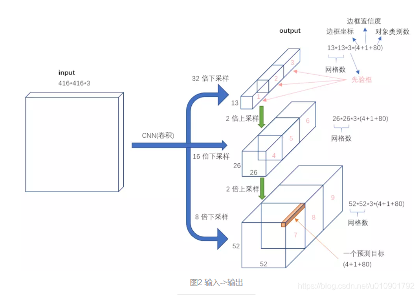
⑤图片输入尺寸，默认为416*416，选择416的原因是：

图片尺寸满足32的倍数，在DarkNet网络中，执行5次步长为2卷积，降采样，其卷积操作如下：
```
x = DarknetConv2D_BN_Leaky(num_filters, (3, 3), strides=(2, 2))(x)
```
- 1
在最底层时，特征图尺寸需要满足为奇数，如13，以保证中心点落在唯一框中。如果为偶数时，则中心点落在中心的4个框中，导致歧义。

创建模型

创建YOLOv3的网络模型，输入：

input_shape：图片尺寸；
anchors：9个anchor box；
num_classes：类别数；
freeze_body：冻结模式，1是冻结DarkNet53的层，2是冻结全部，只保留最后3层；
weights_path：预训练模型的权重。

即：

model = create_model(input_shape, anchors, num_classes,
                     freeze_body=2,
                     weights_path=pretrained_path)

其中，网络的最后3层是：3个1x1的卷积层，用于将3个尺度的特征图，转换为3个尺度的预测值。

即：

out_filters = num_anchors * (num_classes + 5)
// ...
DarknetConv2D(out_filters, (1, 1))

结构如下：

conv2d_59 (Conv2D)      (None, 13, 13, 3*(类别数+4+1))  
conv2d_67 (Conv2D)      (None, 26, 26, 3*(类别数+4+1))  
conv2d_75 (Conv2D)      (None, 52, 52, 3*(类别数+4+1))

模型优化

保存模型

checkpoint = ModelCheckpoint(log_dir + 'ep{epoch:03d}-loss{loss:.3f}-                                                val_loss{val_loss:.3f}.h5',
                             monitor='val_loss', save_weights_only=True,
                             save_best_only=True, period=3)  # 只存储weights权重

学习率

当评价指标不在提升时，减少学习率

 # 当评价指标不在提升时，减少学习率，每次减少10%，当验证损失值，持续3次未减少时，则终止训练。
reduce_lr = ReduceLROnPlateau(monitor='val_loss', factor=0.1, patience=3, verbose=1)

早期停止

验证集准确率下降前终止

monitor：监控数据的类型，支持acc、val_acc、loss、val_loss等；
min_delta：停止阈值，与mode参数配合，支持增加或下降；
mode：min是最少，max是最多，auto是自动，与min_delta配合；
patience：达到阈值之后，能够容忍的epoch数，避免停止在抖动中；
verbose：日志的繁杂程度，值越大，输出的信息越多。

min_delta和patience需要相互配合，避免模型停止在抖动的过程中。min_delta降低，patience减少；而min_delta增加，则patience增加。

#当验证集损失值，连续增加小于0时，持续10个epoch，则终止训练。
early_stopping = EarlyStopping(monitor='val_loss', min_delta=0, patience=10, verbose=1)

注：EarlyStopping是Callback的子类，Callback用于指定在每个阶段开始和结束时，执行的操作。在Callback中，有已经实现的简单子类，如acc、val、loss和val_loss等，还有复杂子类，如ModelCheckpoint和TensorBoard等。

样本数量

样本洗牌，将数据集拆分为10份，训练8份，验证2份，比较简单。

实现：

val_split = 0.2  # 训练和验证的比例with open(annotation_path) as f:
lines = f.readlines()
np.random.seed(47)
np.random.shuffle(lines)
np.random.seed(None)
num_val = int(len(lines) * val_split)  # 验证集数量num_train = len(lines) - num_val  # 训练集数量

训练

损失函数

优化器使用常见的Adam；
损失函数，直接使用模型的输出y_pred，忽略真值y_true；

即：

model.compile(optimizer=Adam(lr=1e-3), loss={
    # 使用定制的 yolo_loss Lambda层
    'yolo_loss': lambda y_true, y_pred: y_pred})  # 损失函数

其中，关于损失函数yolo_loss，以及y_true和y_pred：

把y_true当成输入，作为模型的多输入，把loss封装为层，作为输出；
在模型中，最终输出的y_pred就是loss；
在编译时，将loss设置为y_pred即可，无视y_true；
在训练时，随意添加一个符合结构的y_true即可。

模型fit数据，使用数据生成包装器，按批次生成训练和验证数据。最终，模型model存储权重。

实现如下：

batch_size = 32
model.fit_generator(data_generator_wrapper(lines[:num_train], batch_size, input_shape, anchors, num_classes),
                    steps_per_epoch=max(1, num_train // batch_size),
                    validation_data=data_generator_wrapper(lines[num_train:], batch_size, input_shape, anchors,
                                                           num_classes),
                    validation_steps=max(1, num_val // batch_size),
                    epochs=100,
                    initial_epoch=50,
                    callbacks=[logging, checkpoint, reduce_lr, early_stopping])
model.save_weights(log_dir + 'trained_weights_final.h5')

模型

入口

在训练中，调用create_model方法构建算法模型。

在create_model方法中，创建YOLO v3的算法模型，其中方法参数是：

input_shape：输入图片的尺寸，默认是(416, 416)；
anchors：默认的9种anchor box，结构是(9, 2)；
num_classes：类别个数，在创建网络时，只需类别数即可。在网络中，类别值按0~n排列，同时，输入数据的类别也是用索引表示；
load_pretrained：是否使用预训练权重。预训练权重，既可以产生更好的效果，也可以加快模型的训练速度；
freeze_body：冻结模式，1或2。其中，1是冻结DarkNet53网络中的层，2是只保留最后3个1x1的卷积层，其余层全部冻结；
weights_path：预训练权重的读取路径；

如下：

def create_model(input_shape, anchors, num_classes, load_pretrained=True,      						freeze_body=2,weights_path='model_data/yolo_weights.h5'):

逻辑

在create_model方法中，先将输入参数，进行处理：

拆分图片尺寸的宽h和高w；
创建图片的输入层image_input。在输入层中，既可显式指定图片尺寸，如(416, 416, 3)，也可隐式指定，用“?”代替，如(?, ?, 3)；
计算anchor的数量num_anchors；
根据anchor的数量，创建真值y_true的输入格式。

具体的实现，如下：

h, w = input_shape  # 尺寸
image_input = Input(shape=(w, h, 3))  # 图片输入格式
num_anchors = len(anchors)  # anchor数量

# YOLO的三种尺度，每个尺度的anchor数，类别数+边框4个+置信度1
y_true = [Input(shape=(h // {0: 32, 1: 16, 2: 8}[l], w // {0: 32, 1: 16, 2: 8}[l],
                       num_anchors // 3, num_classes + 5)) for l in range(3)]

其中，真值y_true，真值即Ground Truth。通过循环，创建3个Input层的列表，作为y_true。y_true的张量结构，如下：

Tensor("input_2:0", shape=(?, 13, 13, 3, 5+类别数), dtype=float32)
Tensor("input_3:0", shape=(?, 26, 26, 3, 5+类别数), dtype=float32)
Tensor("input_4:0", shape=(?, 52, 52, 3, 5+类别数), dtype=float32)

其中，在真值y_true中，第1位是输入的样本数，第2~3位是特征图的尺寸，如13x13，第4位是每个图中的anchor数，第5位是：类别(n)+4个框值(x,y,w,h)+框的置信度(是否含有物体)。

接着，通过传入，输入Input层image_input、每个尺度的anchor数num_anchors//3，和类别数num_classes，构建YOLO v3的网络yolo_body，这个yolo_body方法是核心逻辑。

即：

model_body = yolo_body(image_input, num_anchors // 3, num_classes)

下一步，就是加载预训练权重的逻辑块：

根据预训练权重的地址weights_path，加载权重文件，设置参数为，按名称对应by_name，略过不匹配skip_mismatch；
选择冻结模式：模式1是冻结185层。模式2是保留最底部3层，其余全部冻结。整个模型共有252层，185层是DarkNet53网络的层数，而最底部3层是3个1x1的卷积层，用于预测最终结果；将所冻结的层，设置为不可训练，trainable=False；

实现：

if load_pretrained:  # 加载预训练模型
    model_body.load_weights(weights_path, by_name=True, skip_mismatch=True)
    if freeze_body in [1, 2]:
        # Freeze darknet53 body or freeze all but 3 output layers.
        num = (185, len(model_body.layers) - 3)[freeze_body - 1]
        for i in range(num):
            model_body.layers[i].trainable = False  # 将其他层的训练关闭

其中，185层是DarkNet53网络的层数，而最底部3层是3个1x1的卷积层，将3个特征矩阵转换为3个预测矩阵，用于预测最终结果。

其格式如下：

1: (None, 13, 13, 1024) -> (None, 13, 13, 3*(5+类别数))
2: (None, 26, 26, 512) -> (None, 26, 26, 3*(5+类别数))
3: (None, 52, 52, 256) -> (None, 52, 52, 3*(5+类别数))

下一步，构建模型的损失层model_loss，其内容如下：

Lambda是Keras的自定义层，输入为model_body.output和y_true，输出output_shape是(1,)，即一个损失值；
自定义Lambda层的名字name为yolo_loss；
层的参数是锚框列表anchors、类别数num_classes和IoU阈值ignore_thresh。其中，ignore_thresh用于在物体置信度损失中过滤IoU较小的框；
yolo_loss是损失函数的核心逻辑。

实现如下：

model_loss = Lambda(yolo_loss,
				   output_shape=(1,), name='yolo_loss',
                     arguments={'anchors': anchors, 'num_classes': num_classes, 								'ignore_thresh': 0.5})(
        			[*model_body.output, *y_true])

下一步，构建完整的算法模型，步骤如下：

模型的输入层：model_body的输入和真值y_true；
模型的输出层：自定义的model_loss层，其输出是一个损失值(None,1)；

即：

 # 模型
 model = Model(inputs=[model_body.input, *y_true], outputs=model_loss)

其中，model_body.input是任意(?)个(416,416,3)的图片；y_true是已标注数据所转换的真值结构。

即：

[Tensor("input_2:0", shape=(?, 13, 13, 3, 5+num_class), dtype=float32),
  Tensor("input_3:0", shape=(?, 26, 26, 3, 5+num_class), dtype=float32),
  Tensor("input_4:0", shape=(?, 52, 52, 3, 5+num_class), dtype=float32)]

最终，这些逻辑，完成算法模型model的构建。

在这里插入图片描述

网络

在模型中，通过传入输入层image_input、每层的anchor数num_anchors//3和类别数num_classes，调用yolo_body方法，构建YOLO v3的网络model_body。其中，image_input的结构是(?, 416, 416, 3)。

model_body = yolo_body(image_input, num_anchors // 3, num_classes)  # model

在model_body中，最终的输入是image_input，最终的输出是3个矩阵的列表：

[(?, 13, 13, 3*(5+类别数)), 
 (?, 26, 26, 3*(5+类别数)),
 (?, 52, 52, 3*(5+类别数))]

YOLO v3的基础网络是DarkNet网络，将DarkNet网络中底层和中层的特征矩阵，通过卷积操作和多个矩阵的拼接操作，输出3个不同尺度的检测图y1,y2,y3。用于检测不同大小的物体

def yolo_body(inputs, num_anchors, num_classes):
    darknet = Model(inputs, darknet_body(inputs))
    
    x, y1 = make_last_layers(darknet.output, 512, num_anchors * (num_classes + 5))

    x = compose(
        DarknetConv2D_BN_Leaky(256, (1, 1)),
        UpSampling2D(2))(x)
    x = Concatenate()([x, darknet.layers[152].output])
    x, y2 = make_last_layers(x, 256, num_anchors * (num_classes + 5))

    x = compose(
        DarknetConv2D_BN_Leaky(128, (1, 1)),
        UpSampling2D(2))(x)
    x = Concatenate()([x, darknet.layers[92].output])
    x, y3 = make_last_layers(x, 128, num_anchors * (num_classes + 5))

    return Model(inputs, [y1, y2, y3])

Darknet

Darknet网络的输入是图片数据集inputs，即(?, 416, 416, 3)，输出是darknet_body方法的输出。将网络的核心逻辑封装在darknet_body方法中。即：

darknet = Model(inputs, darknet_body(inputs))

其中，darknet_body的输出格式是(?, 13, 13, 1024)。

Darknet的网络简化图，如下：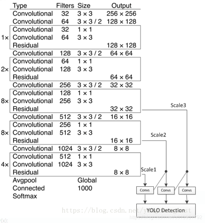
在这里插入图片描述

YOLO v3所使用的Darknet版本是Darknet53。那么，为什么是Darknet53呢？因为Darknet53是53个卷积层和池化层的组合，与Darknet简化图一一对应，即：

53 = 2 + 1*2 + 1 + 2*2 + 1 + 8*2 + 1 + 8*2 + 1 + 4*2 + 1

在darknet_body中，Darknet网络含有5组重复的resblock_body单元，即：

def darknet_body(x):
    '''Darknent body having 52 Convolution2D layers'''
    x = DarknetConv2D_BN_Leaky(32, (3, 3))(x)
    x = resblock_body(x, num_filters=64, num_blocks=1)
    x = resblock_body(x, num_filters=128, num_blocks=2)
    x = resblock_body(x, num_filters=256, num_blocks=8)
    x = resblock_body(x, num_filters=512, num_blocks=8)
    x = resblock_body(x, num_filters=1024, num_blocks=4)
    return x

在第1个卷积操作DarknetConv2D_BN_Leaky中，是3个操作的组合，即：

1个Darknet的2维卷积Conv2D层，即DarknetConv2D；
1个批正在化（BN）层，即BatchNormalization()；
1个LeakyReLU层，斜率是0.1，LeakyReLU是ReLU的变换；

即：

def DarknetConv2D_BN_Leaky(*args, **kwargs):
    """Darknet Convolution2D followed by BatchNormalization and LeakyReLU."""
    no_bias_kwargs = {'use_bias': False}
    no_bias_kwargs.update(kwargs)
    return compose(
        DarknetConv2D(*args, **no_bias_kwargs),
        BatchNormalization(),
        LeakyReLU(alpha=0.1))

其中，Darknet的2维卷积DarknetConv2D，具体操作如下：

将核权重矩阵的正则化，使用L2正则化，参数是5e-4，即操作w参数；
Padding，一般使用same模式，只有当步长为(2,2)时，使用valid模式。避免在降采样中，引入无用的边界信息；
其余参数不变，都与二维卷积操作Conv2D()一致；

kernel_regularizer是将核权重参数w进行正则化，而BatchNormalization是将输入数据x进行正则化。

实现：

@wraps(Conv2D)
def DarknetConv2D(*args, **kwargs):
    """Wrapper to set Darknet parameters for Convolution2D."""
    darknet_conv_kwargs = {'kernel_regularizer': l2(5e-4)}
    darknet_conv_kwargs['padding'] = 'valid' if kwargs.get('strides') == (2, 2) else 'same'
    darknet_conv_kwargs.update(kwargs)
    return Conv2D(*args, **darknet_conv_kwargs)

下一步，第1个残差结构resblock_body，输入的数据x是(?, 416, 416, 32)，通道filters是64个，重复次数num_blocks是1次。第1个残差结构是网络简化图第1部分。

x = resblock_body(x, num_filters=64, num_blocks=1)

在resblock_body中，含有以下逻辑：

ZeroPadding2D：填充x的边界为0，由(?, 416, 416, 32)转换为(?, 417, 417, 32)。因为下一步卷积操作的步长为2，所以图的边长需要是奇数；
DarknetConv2D_BN_Leaky：DarkNet的2维卷积操作，核是(3,3)，步长是(2,2)，注意，这会导致特征尺寸变小，由(?, 417, 417, 32)转换为(?, 208, 208, 64)。由于num_filters是64，所以产生64个通道。
compose：输出预测图y，功能是组合函数，先执行1x1的卷积操作，再执行3x3的卷积操作，filter先降低2倍后恢复，最后与输入相同，都是64；
x = Add()([x, y])：残差（Residual）操作，将x的值与y的值相加。残差操作可以避免，在网络较深时所产生的梯度弥散问题（Vanishing Gradient Problem）。

实现：

def resblock_body(x, num_filters, num_blocks):
    '''A series of resblocks starting with a downsampling Convolution2D'''
    # Darknet uses left and top padding instead of 'same' mode
    x = ZeroPadding2D(((1, 0), (1, 0)))(x)
    x = DarknetConv2D_BN_Leaky(num_filters, (3, 3), strides=(2, 2))(x)
    for i in range(num_blocks):
        y = compose(
            DarknetConv2D_BN_Leaky(num_filters // 2, (1, 1)),
            DarknetConv2D_BN_Leaky(num_filters, (3, 3)))(x)
        x = Add()([x, y])
    return x

残差操作流程，如图：

在这里插入图片描述
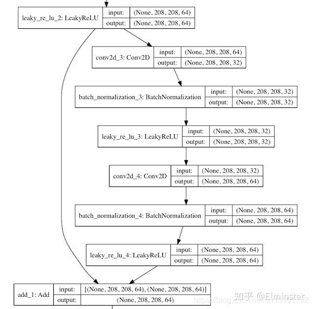
Residual

同理，在darknet_body中，执行5组resblock_body残差块，重复[1, 2, 8, 8, 4]次，双卷积（1x1和3x3）操作，每组均含有一次步长为2的卷积操作，因而一共降维5次32倍，即32=2^5，则输出的特征图维度是13，即13=416/32。最后1层的通道（filter）数是1024，因此，最终的输出结构是(?, 13, 13, 1024)，即：

Tensor("add_23/add:0", shape=(?, 13, 13, 1024), dtype=float32)

至此，Darknet模型的输入是(?, 416, 416, 3)，输出是(?, 13, 13, 1024)。

特征图

在YOLO v3网络中，输出3个不同尺度的检测图，用于检测不同大小的物体。调用3次make_last_layers，产生3个检测图，即y1、y2和y3。

13x13检测图

第1个部分，输出维度是13x13。在make_last_layers方法中，输入参数如下：

darknet.output：DarkNet网络的输出，即(?, 13, 13, 1024)；
num_filters：通道个数512，用于生成中间值x，x会传导至第2个检测图；
out_filters：第1个输出y1的通道数，值是锚框数*(类别数+4个框值+框置信度)；

即：

x, y1 = make_last_layers(darknet.output, 512, num_anchors * (num_classes + 5))

在make_last_layers方法中，执行2步操作：

第1步，x执行多组1x1的卷积操作和3x3的卷积操作，filter先扩大再恢复，最后与输入的filter保持不变，仍为512，则x由(?, 13, 13, 1024)转变为(?, 13, 13, 512)；
第2步，x先执行3x3的卷积操作，再执行不含BN和Leaky的1x1的卷积操作，作用类似于全连接操作，生成预测矩阵y；

Convs由make_last_layers函数来实现。

实现：

def make_last_layers(x, num_filters, out_filters):
    '''6 Conv2D_BN_Leaky layers followed by a Conv2D_linear layer'''
    x = compose(
        DarknetConv2D_BN_Leaky(num_filters, (1, 1)),
        DarknetConv2D_BN_Leaky(num_filters * 2, (3, 3)),
        DarknetConv2D_BN_Leaky(num_filters, (1, 1)),
        DarknetConv2D_BN_Leaky(num_filters * 2, (3, 3)),
        DarknetConv2D_BN_Leaky(num_filters, (1, 1)))(x)
    y = compose(
        DarknetConv2D_BN_Leaky(num_filters * 2, (3, 3)),
        DarknetConv2D(out_filters, (1, 1)))(x)
    return x, y

最终，第1个make_last_layers方法，输出的x是(?, 13, 13, 512)，输出的y是(?, 13, 13, 3*(类别数+5))。

26x26检测图

第2个部分，输出维度是26x26，包含以下步骤：

通过DarknetConv2D_BN_Leaky卷积，将x由512的通道数，转换为256的通道数；
通过2倍上采样UpSampling2D，将x由13x13的结构，转换为26x26的结构；
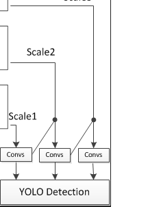
将x与DarkNet的第152层拼接Concatenate，作为第2个make_last_layers的输入，用于生成第2个预测图y2；

其中，输入的x和darknet.layers[152].output的结构都是26x26的尺寸，如下：

x: shape=(?, 26, 26, 256)
darknet.layers[152].output: (?, 26, 26, 512)

在拼接之后，输出的x的格式是(?, 26, 26, 768)。

这样做的目的是：将Darknet最底层的高级抽象信息darknet.output，经过若干次转换之后，除了输出给第1个检测部分，还被用于第2个检测部分，经过上采样，与Darknet骨干中，倒数第2次降维的数据拼接，共同作为第2个检测部分的输入。底层抽象特征含有全局信息，中层抽象特征含有局部信息，这样拼接，两者兼顾，用于检测较小的物体。

在这里插入图片描述

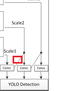
上图红色框图标注的流程实现：

实现：

x = compose(
    DarknetConv2D_BN_Leaky(256, (1, 1)),
    UpSampling2D(2))(x)
x = Concatenate()([x, darknet.layers[152].output])
x, y2 = make_last_layers(x, 256, num_anchors * (num_classes + 5))

最后，还是调用相同的make_last_layers，输出第2个检测层y2和临时数据x。

最终，第2个make_last_layers方法，输出的x是(?, 26, 26, 256)，输出的y是(?, 26, 26, 3*(类别数+4+1))

52x52检测图

第3个部分，输出维度是52x52，与第2个部分类似，包含以下步骤：

x = compose(
    DarknetConv2D_BN_Leaky(128, (1, 1)),
    UpSampling2D(2))(x)
x = Concatenate()([x, darknet.layers[92].output])
_, y3 = make_last_layers(x, 128, num_anchors * (num_classes + 5))

逻辑如下：

x经过128个filter的卷积，再执行上采样，输出为(?, 52, 52, 128)；
darknet.layers[92].output，与152层类似，结构是(?, 52, 52, 256)；
两者拼接之后，x是(?, 52, 52, 384)；
最后输入至make_last_layers，生成y3是(?, 52, 52, 3*(类别数+4+1))，忽略x的输出；

最后，则是根据整个逻辑的输入和输出，构建模型。输入inputs依然保持不变，即(?, 416, 416, 3)，而输出则转换为3个尺度的预测层，即[y1, y2, y3]。

return Model(inputs, [y1, y2, y3])

[y1, y2, y3]的结构如下：

Tensor("conv2d_59/BiasAdd:0", shape=(?, 13, 13, 3*(类别数+4+1)), dtype=float32)
Tensor("conv2d_67/BiasAdd:0", shape=(?, 26, 26, 3*(类别数+4+1)), dtype=float32)
Tensor("conv2d_75/BiasAdd:0", shape=(?, 52, 52, 3*(类别数+4+1)), dtype=float32)

最终，在yolo_body中，完成整个YOLO v3网络的构建，基础网络是DarkNet。

model_body = yolo_body(image_input, num_anchors // 3, num_classes)

总结：

让网络同时学习到深层和浅层的特征，通过叠加浅层特征图相邻特征到不同通道（而非空间位置），类似于Resnet中的identity mapping。这个方法把26x26x512的特征图叠加成13x13x2048的特征图，与原生的深层特征图相连接，使模型有了细粒度特征,增加对小目标的识别能力。

anchor box:

yolov3 anchor box一共有9个，由k-means聚类得到。在COCO数据集上，9个聚类是：

（10,13）（16,30）（33,23）（30,61）（62,45）（59,119）（116,90）（156,198）（373,326）

不同尺寸特征图对应不同大小的先验框。

13*13特征图对应（116,90）（156,198）（373,326）
26*26特征图对应（30,61）（62,45）（59,119）
52*52特征图对应（10,13）（16,30）（33,23）

原因：特征图越大，感受野越小。对小目标越敏感，所以选用小的anchor box。

        特征图越小，感受野越大。对大目标越敏感，所以选用大的anchor box。

真值

fit_generator

在训练中，模型调用fit_generator方法，按批次创建数据，输入模型，进行训练。其中，数据生成器wrapper是data_generator_wrapper，用于验证数据格式，最终调用data_generator，输入参数是：

annotation_lines：标注数据的行，每行数据包含图片路径，和框的位置信息；
batch_size：批次数，每批生成的数据个数；
input_shape：图像输入尺寸，如(416, 416)；
anchors：anchor box列表，9个宽高值；
num_classes：类别的数量；

在data_generator_wrapper中，验证输入参数是否正确，再调用data_generator，这也是wrapper函数的常见用法。

实现：

data_generator_wrapper(lines[:num_train], batch_size, input_shape, anchors, num_classes)

def data_generator_wrapper(annotation_lines, batch_size, input_shape, anchors, num_classes):
    n = len(annotation_lines)  # 标注图片的行数
    if n == 0 or batch_size <= 0: return None
    return data_generator(annotation_lines, batch_size, input_shape, anchors, num_classes)
    
def data_generator(annotation_lines, batch_size, input_shape, anchors, num_classes):

数据生成器

在数据生成器data_generator中，数据的总行数是n，循环输出固定批次数batch_size的图片数据image_data和标注框数据box_data。

在第0次时，将数据洗牌shuffle，调用get_random_data解析annotation_lines[i]，生成图片image和标注框box，添加至各自的列表image_data和box_data中。

索引值递增i+1，当完成n个一轮之后，重新将i置0，再次调用shuffle洗牌数据。

将image_data和box_data都转换为np数组，其中：

image_data: (?, 416, 416, 3)
box_data: (?, 20, 5) # 每个类别最多含有20个框

接着，将框的数据box_data、输入图片尺寸input_shape、anchor box列表anchors和类别数num_classes转换为真值y_true，其中y_true是3个预测特征的列表：

[(?, 13, 13, 3, 5+num_class), (?, 26, 26, 3, 5+num_class), (?, 52, 52, 3, 5+num_class)]

最终输出：图片数据image_data、真值y_true、每个图片的损失值np.zeros。不断循环while True，生成的批次数据，与epoch步数相同，即steps_per_epoch。

实现如下：

def data_generator(annotation_lines, batch_size, input_shape, anchors, num_classes):
    '''data generator for fit_generator'''
    n = len(annotation_lines)
    i = 0
    while True:
        image_data = []
        box_data = []
        for b in range(batch_size):
            if i == 0:
                np.random.shuffle(annotation_lines)
            image, box = get_random_data(annotation_lines[i], input_shape, random=True)  # 获取图片和框
            image_data.append(image)  # 添加图片
            box_data.append(box)  # 添加框
            i = (i + 1) % n
        image_data = np.array(image_data)
        box_data = np.array(box_data)
        y_true = preprocess_true_boxes(box_data, input_shape, anchors, num_classes)  # 真值
        yield [image_data] + y_true, np.zeros(batch_size)

图片和标注框

在get_random_data中，分离图片image和标注框box，输入：

数据annotation_line：图片地址和框的位置类别；
图片尺寸input_shape：如(416, 416)；
数据random：随机开关；

方法如下：

image, box = get_random_data(annotation_lines[i], input_shape, random=True)

def get_random_data(
        annotation_line, input_shape, random=True,
        max_boxes=20, jitter=.3, hue=.1, sat=1.5,
        val=1.5, proc_img=True):

第1步，解析annotation_line数据：

将annotation_line按空格分割为line列表；
使用PIL读取图片image；
图片的宽和高，iw和ih；
输入尺寸的高和宽，h和w；
图片中的标注框box，box是5维，4个点和1个类别；

实现：

line = annotation_line.split()
image = Image.open(line[0])
iw, ih = image.size
h, w = input_shape
box = np.array([np.array(list(map(int, box.split(',')))) for box in line[1:]])

第2步，如果是非随机，即if not random：

将图片等比例转换为416x416的图片，其余用灰色填充，即(128, 128, 128)，同时颜色值转换为0~1之间，即每个颜色值除以255；
将边界框box等比例缩小，再加上填充的偏移量dx和dy，因为新的图片部分用灰色填充，影响box的坐标系，box最多有max_boxes个，即20个。

实现：

scale = min(float(w) / float(iw), float(h) / float(ih))
nw = int(iw * scale)
nh = int(ih * scale)
dx = (w - nw) // 2
dy = (h - nh) // 2
image_data = 0
if proc_img:  # 图片
    image = image.resize((nw, nh), Image.BICUBIC)
    new_image = Image.new('RGB', (w, h), (128, 128, 128))
    new_image.paste(image, (dx, dy))
    image_data = np.array(new_image) / 255.

# 标注框
box_data = np.zeros((max_boxes, 5))
if len(box) > 0:
    np.random.shuffle(box)
    if len(box) > max_boxes: box = box[:max_boxes]  # 最多只取20个
    box[:, [0, 2]] = box[:, [0, 2]] * scale + dx
    box[:, [1, 3]] = box[:, [1, 3]] * scale + dy
    box_data[:len(box)] = box

return image_data, box_data

第3步，如果是随机：

通过jitter参数，随机计算new_ar和scale，生成新的nh和nw，将原始图像随机转换为nw和nh尺寸的图像，即非等比例变换图像。

实现：

new_ar = w / h * rand(1 - jitter, 1 + jitter) / rand(1 - jitter, 1 + jitter)
scale = rand(.25, 2.)
if new_ar < 1:
    nh = int(scale * h)
    nw = int(nh * new_ar)
else:
    nw = int(scale * w)
    nh = int(nw / new_ar)
image = image.resize((nw, nh), Image.BICUBIC)

将变换后的图像，转换为416x416的图像，其余部分用灰色值填充。

实现：

dx = int(rand(0, w - nw))
dy = int(rand(0, h - nh))
new_image = Image.new('RGB', (w, h), (128, 128, 128))
new_image.paste(image, (dx, dy))
image = new_image

根据随机数flip，随机左右翻转FLIP_LEFT_RIGHT图片。

实现：

flip = rand() < .5
if flip: image = image.transpose(Image.FLIP_LEFT_RIGHT)

在HSV坐标域中，改变图片的颜色范围，hue值相加，sat和vat相乘，先由RGB转为HSV，再由HSV转为RGB，添加若干错误判断，避免范围过大。

实现：

hue = rand(-hue, hue)
sat = rand(1, sat) if rand() < .5 else 1 / rand(1, sat)
val = rand(1, val) if rand() < .5 else 1 / rand(1, val)
x = rgb_to_hsv(np.array(image) / 255.)
x[..., 0] += hue
x[..., 0][x[..., 0] > 1] -= 1
x[..., 0][x[..., 0] < 0] += 1
x[..., 1] *= sat
x[..., 2] *= val
x[x > 1] = 1
x[x < 0] = 0
image_data = hsv_to_rgb(x)  # numpy array, 0 to 1

将所有的图片变换，增加至检测框中，并且包含若干异常处理，避免变换之后的值过大或过小，去除异常的box。

实现：

box_data = np.zeros((max_boxes, 5))
if len(box) > 0:
    np.random.shuffle(box)
    box[:, [0, 2]] = box[:, [0, 2]] * nw / iw + dx
    box[:, [1, 3]] = box[:, [1, 3]] * nh / ih + dy
    if flip: box[:, [0, 2]] = w - box[:, [2, 0]]
    box[:, 0:2][box[:, 0:2] < 0] = 0
    box[:, 2][box[:, 2] > w] = w
    box[:, 3][box[:, 3] > h] = h
    box_w = box[:, 2] - box[:, 0]
    box_h = box[:, 3] - box[:, 1]
    box = box[np.logical_and(box_w > 1, box_h > 1)]  # discard invalid box
    if len(box) > max_boxes: box = box[:max_boxes]
    box_data[:len(box)] = box

最终，返回图像数据image_data和边框数据box_data。box的4个值是(xmin, ymin, xmax, ymax)，第5位不变，是标注框的类别，如0~n。

真值y_true

在preprocess_true_boxes中，输入：

true_boxes：检测框，批次数?，最大框数20，每个框5个值，4个边界点和1个类别序号，如(?, 20, 5)；
input_shape：图片尺寸，如(416, 416)；
anchors：anchor box列表；
num_classes：类别的数量；

如：

def preprocess_true_boxes(true_boxes, input_shape, anchors, num_classes):

检测类别序号是否小于类别数，避免异常数据，如：

assert (true_boxes[..., 4] < num_classes).all(), 'class id must be less than num_classes'

每一层anchor box的数量num_layers；

预设anchor box的掩码anchor_mask，第1层678，第2层345，第3层012，倒序排列。

实现：

num_layers = len(anchors) // 3  # default setting
anchor_mask = [[6, 7, 8], [3, 4, 5], [0, 1, 2]] if num_layers == 3 else [[3, 4, 5], [1, 2, 3]]

计算true_boxes：

true_boxes：真值框，左上和右下2个坐标值和1个类别，如[184, 299, 191, 310, 0.0]，结构是(?, 20, 5)，?是批次数，20是框的最大数，5是框的5个值；
boxes_xy：xy是box的中心点，结构是(?, 20, 2)；
boxes_wh：wh是box的宽和高，结构也是(?, 20, 2)；
input_shape：输入尺寸416x416；

true_boxes：第0和1位设置为xy，除以416，归一化，第2和3位设置为wh，除以416，归一化，如[0.449, 0.730, 0.016, 0.026, 0.0]。

实现：

true_boxes = np.array(true_boxes, dtype='float32')
input_shape = np.array(input_shape, dtype='int32')
boxes_xy = (true_boxes[..., 0:2] + true_boxes[..., 2:4]) // 2
boxes_wh = true_boxes[..., 2:4] - true_boxes[..., 0:2]
true_boxes[..., 0:2] = boxes_xy / input_shape[::-1]
true_boxes[..., 2:4] = boxes_wh / input_shape[::-1]

设置y_true的初始值：

m是批次；
grid_shape是input_shape等比例降低，即[[13,13], [26,26], [52,52]]；
y_true是全0矩阵（np.zeros）列表，即:

[(?,13,13,3,5+num_class),

(?,26,26,3,5+num_class),

(?,52,52,3,5+num_class)]

实现：

m = true_boxes.shape[0]
grid_shapes = [input_shape // {0: 32, 1: 16, 2: 8}[l] for l in range(num_layers)]
y_true = [np.zeros((m, grid_shapes[l][0], grid_shapes[l][1], len(anchor_mask[l]), 5 +              num_classes),dtype='float32') for l in range(num_layers)]

设置anchors的值：

将anchors增加1维expand_dims，由(9,2)转为(1,9,2)；
anchor_maxes，是anchors值除以2；
anchor_mins，是负的anchor_maxes；
valid_mask，将boxes_wh中宽w大于0的位，设为True，即含有box，结构是(?,20)；

valid_mask：

实现：

anchors = np.expand_dims(anchors, 0)
anchor_maxes = anchors / 2.
anchor_mins = -anchor_maxes
valid_mask = boxes_wh[..., 0] > 0

循环m处理批次中的每个图像和标注框：

只选择存在标注框的wh，例如：wh的shape是(1,2)
np.expand_dims(wh, -2)是wh倒数第2个添加1位，即(1,2)->(1,1,2)；
box_maxes和box_mins，与anchor_maxes和anchor_mins的操作类似。

实现：

for b in range(m):
    # Discard zero rows.
    wh = boxes_wh[b, valid_mask[b]]
    if len(wh) == 0: continue
    # Expand dim to apply broadcasting.
    wh = np.expand_dims(wh, -2)
    box_maxes = wh / 2.
    box_mins = -box_maxes

计算标注框box与anchor box的iou值，计算方式很巧妙：

box_mins的shape是(1,1,2)，anchor_mins的shape是(1,9,2)，intersect_mins的shape是(1,9,2)，即两两组合的值；
intersect_area的shape是(1,9)；box_area的shape是(1,1)；anchor_area的shape是(1,9)；
iou的shape是(1,9)；

IoU数据，即anchor box与检测框box，两两匹配的iou值。

实现：

intersect_mins = np.maximum(box_mins, anchor_mins)
intersect_maxes = np.minimum(box_maxes, anchor_maxes)
intersect_wh = np.maximum(intersect_maxes - intersect_mins, 0.)
intersect_area = intersect_wh[..., 0] * intersect_wh[..., 1]
box_area = wh[..., 0] * wh[..., 1]
anchor_area = anchors[..., 0] * anchors[..., 1]
iou = intersect_area / (box_area + anchor_area - intersect_area)

接着，选择IoU最大的anchor索引，即：

best_anchor = np.argmax(iou, axis=-1)

设置y_true的值：

t是box的序号；n是最优anchor的序号；l是层号；
如果最优anchor在层l中，则设置其中的值，否则默认为0；
true_boxes是(?, 20, 5)，即批次、box数、框值；
true_boxes[b, t, 0]，其中b是批次序号、t是box序号，第0位是x，第1位是y；
grid_shapes是3个检测图的尺寸，将归一化的值，与框长宽相乘，恢复为具体值；
k是在anchor box中的序号；
c是类别，true_boxes的第4位；
将xy和wh放入y_true中，将y_true的第4位框的置信度设为1，第5~n位的类别设为1；

实现：

for t, n in enumerate(best_anchor):
    for l in range(num_layers):
        if n in anchor_mask[l]:
            i = np.floor(true_boxes[b, t, 0] * grid_shapes[l][1]).astype('int32')
            j = np.floor(true_boxes[b, t, 1] * grid_shapes[l][0]).astype('int32')
            k = anchor_mask[l].index(n)
            c = true_boxes[b, t, 4].astype('int32')
            y_true[l][b, j, i, k, 0:4] = true_boxes[b, t, 0:4]
            y_true[l][b, j, i, k, 4] = 1
            y_true[l][b, j, i, k, 5 + c] = 1

y_true的第0和1位是中心点xy，范围是(0~1)，第2和3位是宽高wh，范围是0~1，第4位是置信度1或0，第5~n位是类别为1其余为0。

Loss

损失层

在模型的训练过程中，不断调整网络中的参数，优化损失函数loss的值达到最小，完成模型的训练。在YOLO v3中，损失函数yolo_loss封装自定义Lambda的损失层中，作为模型的最后一层，参于训练。损失层Lambda的输入是已有模型的输出model_body.output和真值y_true，输出是1个值，即损失值。

损失层的核心逻辑位于yolo_loss中，yolo_loss除了接收Lambda层的输入model_body.output和y_true，还接收锚框anchors、类别数num_classes和过滤阈值ignore_thresh等3个参数。

实现：

model_loss = Lambda(yolo_loss,
                    output_shape=(1,), name='yolo_loss',
                    arguments={'anchors': anchors,
                               'num_classes': num_classes,
                               'ignore_thresh': 0.5}
                    )([*model_body.output, *y_true])

其中，model_body.output是已有模型的预测值，y_true是真实值，两者的格式相同，如下：

model_body.output: [(?, 13, 13, 3*(5+num_class)), 
                    (?, 26, 26, 3*(5+num_class)),
                    (?, 52, 52, 3*(5+num_class))]
y_true: [(?, 13, 13, 3*(5+num_class)), 
         (?, 26, 26, 3*(5+num_class)),
         (?, 52, 52, 3*(5+num_class))]

接着，在yolo_loss方法中，参数是：

args是Lambda层的输入，即model_body.output和y_true的组合；
anchors是二维数组，结构是(9, 2)，即9个anchor box；
num_classes是类别数；
ignore_thresh是过滤阈值；
print_loss是打印损失函数的开关；

即：

def yolo_loss(args, anchors, num_classes, ignore_thresh=.5, print_loss=True):

参数

在损失方法yolo_loss中，设置若干参数：

num_layers：层的数量；
yolo_outputs和y_true：分离args，前3个是yolo_outputs预测值，后3个是y_true真值；
anchor_mask：anchor box的索引数组，3个1组倒序排序，678对应13x13，345对应26x26，123对应52x52；即[[6, 7, 8], [3, 4, 5], [0, 1, 2]]；
input_shape：K.shape(yolo_outputs[0])[1:3]，第1个预测矩阵yolo_outputs[0]的结构（shape）的第1~2位，即

(?, 13, 13, 3*(5+num_class))中的(13, 13)。再x32，就是YOLO网络的输入尺寸，即(416, 416)，因为在网络中，含有5个步长为(2, 2)的卷积操作，降维32=5^2倍；
grid_shapes：与input_shape类似，K.shape()[1:3]，以列表的形式，选择3个尺寸的预测图维度，即[(13, 13), (26, 26), (52, 52)]；
m：第1个预测图的结构的第1位，即K.shape()[0]，输入模型的图片总量，即批次数；
mf：m的float类型，即K.cast(m, K.dtype())
loss：损失值为0；

即：

num_layers = len(anchors) // 3  # default setting
yolo_outputs = args[:num_layers]
y_true = args[num_layers:]
anchor_mask = [[6, 7, 8], [3, 4, 5], [0, 1, 2]] if num_layers == 3 else [[3, 4, 5], [1, 2, 3]]
# input_shape是输出的尺寸*32, 就是原始的输入尺寸，[1:3]是尺寸的位置，即416x416
input_shape = K.cast(K.shape(yolo_outputs[0])[1:3] * 32, K.dtype(y_true[0]))
# 每个网格的尺寸，组成列表
grid_shapes = [K.cast(K.shape(yolo_outputs[l])[1:3], K.dtype(y_true[0])) for l in range(num_layers)]

m = K.shape(yolo_outputs[0])[0]  # batch size, tensor
mf = K.cast(m, K.dtype(yolo_outputs[0]))

loss = 0

预测数据

在yolo_head中，将预测图yolo_outputs[l]，拆分为边界框的起始点xy、宽高wh、置信度confidence和类别概率class_probs。输入参数：

yolo_outputs[l]或feats：第l个预测图，如(?, 13, 13, 3(5+num_class))；
anchors[anchor_mask[l]]或anchors：第l层anchor box，如[(116, 90), (156,198), (373,326)]；
num_classes：类别数，如1个；
input_shape：输入图片的尺寸，Tensor，值为(416, 416)；
calc_loss：计算loss的开关，在计算损失值时，calc_loss打开，为True；

即：

grid, raw_pred, pred_xy, pred_wh = \    
    yolo_head(yolo_outputs[l], anchors[anchor_mask[l]], num_classes, input_shape, calc_loss=True)
    
def yolo_head(feats, anchors, num_classes, input_shape, calc_loss=False):

接着，统计anchors的数量num_anchors，即3个。将anchors转换为与预测图feats维度相同的Tensor，即anchors_tensor的结构是(1, 1, 1, 3, 2)，即：

num_anchors = len(anchors)
# Reshape to batch, height, width, num_anchors, box_params.
anchors_tensor = K.reshape(K.constant(anchors), [1, 1, 1, num_anchors, 2])

下一步，创建网格grid：

获取网格的尺寸grid_shape，即预测图feats的第1~2位，如13x13；
grid_y和grid_x用于生成网格grid，通过arange、reshape、tile的组合，创建y轴的0~12的组合grid_y，再创建x轴的0~12的组合grid_x，将两者拼接concatenate，就是grid；
grid是遍历二元数值组合的数值，结构是(13, 13, 1, 2)；

即：

grid_shape = K.shape(feats)[1:3]
grid_shape = K.shape(feats)[1:3]  # height, width
grid_y = K.tile(K.reshape(K.arange(0, stop=grid_shape[0]), [-1, 1, 1, 1]),
                [1, grid_shape[1], 1, 1])
grid_x = K.tile(K.reshape(K.arange(0, stop=grid_shape[1]), [1, -1, 1, 1]),
                [grid_shape[0], 1, 1, 1])
grid = K.concatenate([grid_x, grid_y])
grid = K.cast(grid, K.dtype(feats))

下一步，将feats的最后一维展开，将anchors与其他数据（类别数+4个框值+框置信度）分离

feats = K.reshape(
    feats, [-1, grid_shape[0], grid_shape[1], num_anchors, num_classes + 5])

下一步，计算起始点xy、宽高wh、框置信度box_confidence和类别置信度box_class_probs：

起始点xy：将feats中xy的值，经过sigmoid归一化，再加上相应的grid的二元组，再除以网格边长，归一化；
宽高wh：将feats中wh的值，经过exp正值化，再乘以anchors_tensor的anchor box，再除以图片宽高，归一化；
框置信度box_confidence：将feats中confidence值，经过sigmoid归一化；
类别置信度box_class_probs：将feats中class_probs值，经过sigmoid归一化；

即：

box_xy = (K.sigmoid(feats[..., :2]) + grid) / K.cast(grid_shape[::-1], K.dtype(feats))
box_wh = K.exp(feats[..., 2:4]) * anchors_tensor / K.cast(input_shape[::-1], K.dtype(feats))
box_confidence = K.sigmoid(feats[..., 4:5])
box_class_probs = K.sigmoid(feats[..., 5:])

其中，xywh的计算公式，tx、ty、tw和th是feats值，而bx、by、bw和bh是输出值，如下：

框的4个值

这4个值box_xy, box_wh, confidence, class_probs的范围均在0~1之间。

由于计算损失值，calc_loss为True，则返回：

网格grid：结构是(13, 13, 1, 2)，数值为0~12的全遍历二元组；
预测值feats：经过reshape变换，将18维数据分离出3维anchors，结构是(?, 13, 13, 3, 6)
box_xy和box_wh归一化的起始点xy和宽高wh，xy的结构是(?, 13, 13, 3, 2)，wh的结构是(?, 13, 13, 3, 2)；box_xy的范围是(0~1)，box_wh的范围是(0~1)；即bx、by、bw、bh计算完成之后，再进行归一化。

即：

if calc_loss == True:
    return grid, feats, box_xy, box_wh

损失函数

在计算损失值时，循环计算每1层的损失值，累加到一起，即

for l in range(num_layers):
        // ... 
        loss += xy_loss + wh_loss + confidence_loss + class_loss

在每个循环体中：

获取物体置信度object_mask，最后1个维度的第4位，第0~3位是框，第4位是物体置信度；
类别置信度true_class_probs，最后1个维度的第5位；

即：

object_mask = y_true[l][..., 4:5]
true_class_probs = y_true[l][..., 5:]

接着，调用yolo_head重构预测图，输出：

网格grid：l=0时，结构是(13, 13, 1, 2)，数值为0~12的全遍历二元组；
预测值raw_pred：经过reshape变换，将anchors分离，结构是(?, 13, 13, 3, 5+类别数)
pred_xy和pred_wh归一化的起始点xy和宽高wh，xy的结构是(?, 13, 13, 3, 2)，wh的结构是(?, 13, 13, 3, 2)；

再将xy和wh组合成预测框pred_box，结构是(?, 13, 13, 3, 4)。

grid, raw_pred, pred_xy, pred_wh = \   
    yolo_head(yolo_outputs[l], anchors[anchor_mask[l]], 
              num_classes, input_shape, calc_loss=True)
pred_box = K.concatenate([pred_xy, pred_wh])

接着，生成真值数据：

raw_true_xy：在网格中的中心点xy，偏移数据，值的范围是0~1；y_true的第0和1位是中心点xy的相对位置，范围是0~1；
raw_true_wh：在网络中的wh针对于anchors的比例，再转换为log形式，范围是有正有负；y_true的第2和3位是宽高wh的相对位置，范围是0~1；
box_loss_scale：计算wh权重，取值范围(1~2)；

实现：

# Darknet raw box to calculate loss.
raw_true_xy = y_true[l][..., :2] * grid_shapes[l][::-1] - grid
raw_true_wh = K.log(y_true[l][..., 2:4] / anchors[anchor_mask[l]] * input_shape[::-1])  # 1
raw_true_wh = K.switch(object_mask, raw_true_wh, K.zeros_like(raw_true_wh))  # avoid log(0)=-inf
box_loss_scale = 2 - y_true[l][..., 2:3] * y_true[l][..., 3:4]  # 2-w*h

接着，根据IoU忽略阈值生成ignore_mask，将预测框pred_box和真值框true_box计算IoU，抑制不需要的anchor框的值，即IoU小于最大阈值的anchor框。ignore_mask的shape是(?, ?, ?, 3, 1)，第0位是批次数，第1~2位是特征图尺寸。

实现：

ignore_mask = tf.TensorArray(K.dtype(y_true[0]), size=1, dynamic_size=True)
object_mask_bool = K.cast(object_mask, 'bool')

def loop_body(b, ignore_mask):
    true_box = tf.boolean_mask(y_true[l][b, ..., 0:4], object_mask_bool[b, ..., 0])
    iou = box_iou(pred_box[b], true_box)
    best_iou = K.max(iou, axis=-1)
    ignore_mask = ignore_mask.write(b, K.cast(best_iou < ignore_thresh, K.dtype(true_box)))
    return b + 1, ignore_mask

_, ignore_mask = K.control_flow_ops.while_loop(lambda b, *args: b < m, loop_body, [0, ignore_mask])
ignore_mask = ignore_mask.stack()
ignore_mask = K.expand_dims(ignore_mask, -1)

损失函数：

xy_loss：中心点的损失值。

object_mask是y_true的第4位，即是否含有物体，含有是1，不含是0。

box_loss_scale的值，与物体框的大小有关，2减去相对面积，值得范围是(1~2)。binary_crossentropy是二值交叉熵。
wh_loss：宽高的损失值。除此之外，额外乘以系数0.5，平方K.square()。
confidence_loss：框的损失值。两部分组成，第1部分是存在物体的损失值，第2部分是不存在物体的损失值，其中乘以忽略掩码ignore_mask，忽略预测框中IoU大于阈值的框。
class_loss：类别损失值。
将各部分损失值的和，除以均值，累加，作为最终的图片损失值。

细节实现：

object_mask = y_true[l][..., 4:5]  # 物体掩码
box_loss_scale = 2 - y_true[l][..., 2:3] * y_true[l][..., 3:4]  # 框损失比例
z * -log(sigmoid(x)) + (1 - z) * -log(1 - sigmoid(x))  # 二值交叉熵函数
iou = box_iou(pred_box[b], true_box)  # 预测框与真正框的IoU

损失函数实现：

xy_loss = object_mask * box_loss_scale * K.binary_crossentropy(raw_true_xy, raw_pred[..., 0:2],
                                                               from_logits=True)
wh_loss = object_mask * box_loss_scale * 0.5 * K.square(raw_true_wh - raw_pred[..., 2:4])
confidence_loss = object_mask * K.binary_crossentropy(object_mask, raw_pred[..., 4:5], from_logits=True) + \                 
                  (1 - object_mask) * K.binary_crossentropy(object_mask, raw_pred[..., 4:5],
                                                            from_logits=True) * ignore_mask
class_loss = object_mask * K.binary_crossentropy(true_class_probs, raw_pred[..., 5:], from_logits=True)

xy_loss = K.sum(xy_loss) / mf
wh_loss = K.sum(wh_loss) / mf
confidence_loss = K.sum(confidence_loss) / mf
class_loss = K.sum(class_loss) / mf
loss += xy_loss + wh_loss + confidence_loss + class_loss

YOLO v1的损失函数公式，与v3略有不同，作为参考：

预测

检测函数

使用已经训练完成的YOLO v3模型，检测图片中的物体，其中：

创建YOLO类的实例yolo；
使用Image.open()加载图像image；
调用yolo.detect_image()检测图像image；
关闭yolo的session；
显示检测完成的图像r_image；

实现：

def detect_img_for_test():
    yolo = YOLO()
    img_path = './dataset/img.jpg'
    image = Image.open(img_path)
    r_image = yolo.detect_image(image)
    yolo.close_session()
    r_image.show()

输出：

YOLO参数

YOLO类的初始化参数：

anchors_path：anchor box的配置文件，9个宽高组合；
model_path：已训练完成的模型，支持重新训练的模型；
classes_path：类别文件，与模型文件匹配；
score：置信度的阈值，删除小于阈值的候选框；
iou：候选框的IoU阈值，删除同类别中大于阈值的候选框；
class_names：类别列表，读取classes_path；
anchors：anchor box列表，读取anchors_path；
model_image_size：模型所检测图像的尺寸，输入图像都需要按此填充；
colors：通过HSV色域，生成随机颜色集合，数量等于类别数class_names；
boxes、scores、classes：检测的核心输出，函数generate()所生成，是模型的输出封装。

实现：

self.anchors_path = 'configs/yolo_anchors.txt'  # Anchors
self.model_path = 'model_data/yolo_weights.h5'  # 模型文件
self.classes_path = 'configs/coco_classes.txt'  # 类别文件

self.score = 0.50
self.iou = 0.20
self.class_names = self._get_class()  # 获取类别
self.anchors = self._get_anchors()  # 获取anchor
self.sess = K.get_session()
self.model_image_size = (416, 416)  # fixed size or (None, None), hw
self.colors = self.__get_colors(self.class_names)
self.boxes, self.scores, self.classes = self.generate()

在__get_colors()中：

将HSV的第0位H值，按1等分，其余SV值，均为1，生成一组HSV列表；
调用hsv_to_rgb，将HSV色域转换为RGB色域；
0~1的RGB值乘以255，转换为完整的颜色值，(0~255)；
随机shuffle颜色列表；

实现：

@staticmethod def __get_colors(names):
    # 不同的框，不同的颜色
    hsv_tuples = [(float(x) / len(names), 1., 1.)
                  for x in range(len(names))]  # 不同颜色
    colors = list(map(lambda x: colorsys.hsv_to_rgb(*x), hsv_tuples))
    colors = list(map(lambda x: (int(x[0] * 255), int(x[1] * 255), int(x[2] * 255)), colors))  # RGB
    np.random.seed(10101)
    np.random.shuffle(colors)
    np.random.seed(None)

    return colors

选择HSV划分，而不是RGB的原因是，HSV的颜色值偏移更好，画出的框，颜色更容易区分。

输出封装

boxes、scores、classes是在模型的基础上，继续封装，由函数generate()所生成，其中：

boxes：框的四个点坐标，(top, left, bottom, right)；
scores：框的类别置信度，融合框置信度和类别置信度；
classes：框的类别；

在函数generate()中，设置参数：

num_anchors：anchor box的总数，一般是9个；
num_classes：类别总数，如COCO是80个类；
yolo_model：由yolo_body所创建的模型，调用load_weights加载参数；

实现：

num_anchors = len(self.anchors)  # anchors的数量
num_classes = len(self.class_names)  # 类别数

self.yolo_model = yolo_body(Input(shape=(416, 416, 3)), 3, num_classes)
self.yolo_model.load_weights(model_path)  # 加载模型参数

接着，设置input_image_shape为placeholder，即TF中的参数变量。在yolo_eval中：

继续封装yolo_model的输出output；
anchors，anchor box列表；
类别class_names的总数len()；
输入图片的可选尺寸，input_image_shape，即(416, 416)；
score_threshold，框的整体置信度阈值score；
iou_threshold，同类别框的IoU阈值iou；
返回，框的坐标boxes，框的类别置信度scores，框的类别classes；

实现：

self.input_image_shape = K.placeholder(shape=(2,))
boxes, scores, classes = yolo_eval(
    self.yolo_model.output, self.anchors, len(self.class_names),
    self.input_image_shape, score_threshold=self.score, iou_threshold=self.iou)
return boxes, scores, classes

输出的scores值，都会大于score_threshold，小于的在yolo_eval()中已被删除。

YOLO评估

在函数yolo_eval()中，完成预测逻辑的封装，其中输入：

yolo_outputs：YOLO模型的输出，3个尺度的列表，即13-26-52，最后1维是预测值，由3x(5+num_class)组成，3是每层的anchor数，5是4个框值xywh和1个框中含有物体的置信度，num_class是类别数；
anchors：9个anchor box的值；
num_classes：类别个数；
image_shape：placeholder类型的TF参数，默认(416, 416)；
max_boxes：图中最大的检测框数，20个；
score_threshold：框置信度阈值，小于阈值的框被删除，需要的框较多，则调低阈值，需要的框较少，则调高阈值；
iou_threshold：同类别框的IoU阈值，大于阈值的重叠框被删除，重叠物体较多，则调高阈值，重叠物体较少，则调低阈值；

其中，yolo_outputs格式，如下：

[(?, 13, 13, 3x(5+num_class)), 
(?, 26, 26, 3x(5+num_class)), 
(?, 52, 52, 3x(5+num_class))]

其中，anchors列表，如下：

[(10,13), (16,30), (33,23), (30,61), (62,45), (59,119), (116,90), (156,198), (373,326)]

实现：

boxes, scores, classes = yolo_eval(
    self.yolo_model.output, self.anchors, len(self.class_names),
    self.input_image_shape, score_threshold=self.score, iou_threshold=self.iou)

def yolo_eval(yolo_outputs, anchors, num_classes, image_shape,
              max_boxes=20, score_threshold=.6, iou_threshold=.5):

接着，处理参数：

num_layers，输出特征图的层数，3层；
anchor_mask，将anchors划分为3个层，第1层13x13是678，第2层26x26是345，第3层52x52是012；
input_shape：输入图像的尺寸，也就是第0个特征图的尺寸乘以32，即13x32=416，这与Darknet的网络结构有关。

num_layers = len(yolo_outputs)
anchor_mask = [[6, 7, 8], [3, 4, 5], [0, 1, 2]] if num_layers == 3 else [[3, 4, 5], [1, 2, 3]]  # default setting
input_shape = K.shape(yolo_outputs[0])[1:3] * 32

特征图越大，13->52，检测的物体越小，需要的anchors越小，所以anchors列表以倒序赋值。

接着，在YOLO的第l层输出yolo_outputs中，调用yolo_boxes_and_scores()，提取框_boxes和置信度_box_scores，将3个层的框数据放入列表boxes和box_scores，再拼接concatenate展平，输出的数据就是所有的框和置信度。

其中，输出的boxes和box_scores的格式，如下：

boxes: (?, 4)  # ?是框数
box_scores: (?, num_class)#框置信度与类别置信度的乘积

实现：

boxes = []
box_scores = []
for l in range(num_layers):
    _boxes, _box_scores = yolo_boxes_and_scores(
        yolo_outputs[l], anchors[anchor_mask[l]], num_classes, input_shape, image_shape)
    boxes.append(_boxes)
    box_scores.append(_box_scores)
boxes = K.concatenate(boxes, axis=0)
box_scores = K.concatenate(box_scores, axis=0)

concatenate的作用是：将多个层的数据展平，因为框已经还原为真实坐标，不同尺度没有差异。

在函数yolo_boxes_and_scores()中：

yolo_head的输出：box_xy是box的中心坐标，(0~1)相对位置；box_wh是box的宽高，(0~1)相对值；box_confidence是框中物体置信度；box_class_probs是类别置信度；
yolo_correct_boxes，将box_xy和box_wh的(0~1)相对值，转换为真实坐标，输出boxes是(y_min,x_min,y_max,x_max)的值；
reshape，将不同网格的值展平为框的列表，即(?,13,13,3,4)->(?,4)；
box_scores是框置信度与类别置信度的乘积，再reshape展平，(?,num_class)；
返回框boxes和框置信度box_scores。

实现：

def yolo_boxes_and_scores(feats, anchors, num_classes, input_shape, image_shape):
    '''Process Conv layer output'''
    box_xy, box_wh, box_confidence, box_class_probs = yolo_head(
        feats, anchors, num_classes, input_shape)
    boxes = yolo_correct_boxes(box_xy, box_wh, input_shape, image_shape)
    boxes = K.reshape(boxes, [-1, 4])
    box_scores = box_confidence * box_class_probs
    box_scores = K.reshape(box_scores, [-1, num_classes])
    return boxes, box_scores

接着：

mask，过滤小于置信度阈值的框，只保留大于置信度的框，mask掩码；
max_boxes_tensor，每个类别最大检测框数，max_boxes是20；

实现：

mask = box_scores >= score_threshold
max_boxes_tensor = K.constant(max_boxes, dtype='int32')

接着：

通过掩码mask和类别c，筛选框class_boxes和置信度class_box_scores；
通过NMS，非极大值抑制，筛选出框boxes的NMS索引nms_index；
根据索引，选择gather输出的框class_boxes和置信class_box_scores度，再生成类别信息classes；
将多个类别的数据组合，生成最终的检测数据框，并返回。

实现：

boxes_ = []
scores_ = []
classes_ = []
for c in range(num_classes):
    class_boxes = tf.boolean_mask(boxes, mask[:, c])
    class_box_scores = tf.boolean_mask(box_scores[:, c], mask[:, c])
    nms_index = tf.image.non_max_suppression(
        class_boxes, class_box_scores, max_boxes_tensor, iou_threshold=iou_threshold)
    class_boxes = K.gather(class_boxes, nms_index)
    class_box_scores = K.gather(class_box_scores, nms_index)
    classes = K.ones_like(class_box_scores, 'int32') * c
    boxes_.append(class_boxes)
    scores_.append(class_box_scores)
    classes_.append(classes)
boxes_ = K.concatenate(boxes_, axis=0)
scores_ = K.concatenate(scores_, axis=0)
classes_ = K.concatenate(classes_, axis=0)

输出格式：

boxes_: (?, 4)
scores_: (?,)
classes_: (?,)

检测方法

第1步，图像处理：

将图像等比例转换为检测尺寸，检测尺寸需要是32的倍数，周围进行填充；
将图片增加1维，符合输入参数格式；

if self.model_image_size != (None, None):  # 416x416, 416=32*13，必须为32的倍数，最小尺度是除以32
    assert self.model_image_size[0] % 32 == 0, 'Multiples of 32 required'
    assert self.model_image_size[1] % 32 == 0, 'Multiples of 32 required'
    boxed_image = letterbox_image(image, tuple(reversed(self.model_image_size)))  # 填充图像
else:
    new_image_size = (image.width - (image.width % 32), image.height - (image.height % 32))
    boxed_image = letterbox_image(image, new_image_size)
image_data = np.array(boxed_image, dtype='float32')
print('detector size {}'.format(image_data.shape))
image_data /= 255.  # 转换0~1
image_data = np.expand_dims(image_data, 0)  # 添加批次维度，将图片增加1维

第2步，feed数据，图像，图像尺寸；

out_boxes, out_scores, out_classes = self.sess.run(
    [self.boxes, self.scores, self.classes],
    feed_dict={
        self.yolo_model.input: image_data,
        self.input_image_shape: [image.size[1], image.size[0]],
        K.learning_phase(): 0
    })

第3步，绘制边框，自动设置边框宽度，绘制边框和类别文字，使用Pillow绘图库。

font = ImageFont.truetype(font='font/FiraMono-Medium.otf',
                          size=np.floor(3e-2 * image.size[1] + 0.5).astype('int32'))  # 字体
thickness = (image.size[0] + image.size[1]) // 512  # 厚度
for i, c in reversed(list(enumerate(out_classes))):
    predicted_class = self.class_names[c]  # 类别
    box = out_boxes[i]  # 框
    score = out_scores[i]  # 执行度

    label = '{} {:.2f}'.format(predicted_class, score)  # 标签
    draw = ImageDraw.Draw(image)  # 画图
    label_size = draw.textsize(label, font)  # 标签文字

    top, left, bottom, right = box
    top = max(0, np.floor(top + 0.5).astype('int32'))
    left = max(0, np.floor(left + 0.5).astype('int32'))
    bottom = min(image.size[1], np.floor(bottom + 0.5).astype('int32'))
    right = min(image.size[0], np.floor(right + 0.5).astype('int32'))
    print(label, (left, top), (right, bottom))  # 边框

    if top - label_size[1] >= 0:  # 标签文字
        text_origin = np.array([left, top - label_size[1]])
    else:
        text_origin = np.array([left, top + 1])

    # My kingdom for a good redistributable image drawing library.
    for i in range(thickness):  # 画框
        draw.rectangle(
            [left + i, top + i, right - i, bottom - i],
            outline=self.colors[c])
    draw.rectangle(  # 文字背景
        [tuple(text_origin), tuple(text_origin + label_size)],
        fill=self.colors[c])
    draw.text(text_origin, label, fill=(0, 0, 0), font=font)  # 文案
    del draw

补充

1. IoU

IoU，即Intersection over Union，用于计算两个图的重叠度，用于计算两个标注框之间的相关度，值越高，相关度越高。在NMS非极大值抑制或计算mAP中，都会使用IoU判断两个框的相关性。

如图：

实现：

def bb_intersection_over_union(boxA, boxB):
    boxA = [int(x) for x in boxA]
    boxB = [int(x) for x in boxB]

    xA = max(boxA[0], boxB[0])
    yA = max(boxA[1], boxB[1])
    xB = min(boxA[2], boxB[2])
    yB = min(boxA[3], boxB[3])

    interArea = max(0, xB - xA + 1) * max(0, yB - yA + 1)

    boxAArea = (boxA[2] - boxA[0] + 1) * (boxA[3] - boxA[1] + 1)
    boxBArea = (boxB[2] - boxB[0] + 1) * (boxB[3] - boxB[1] + 1)
    
    iou = interArea / float(boxAArea + boxBArea - interArea)

    return iou

2. 冻结网络层

在微调中，需要确定冻结的层数和可训练的层数，主要取决于，数据集相似度和新数据集的大小。原则上，相似度越高，则固定的层数越多；新数据集越大，不考虑训练时间的成本，则可训练更多的层数。然后可能也要考虑数据集本身的类别间差异度，但上面说的规则基本上还是成立的。

例如，在图片分类的网络中，底层一般是颜色、轮廓、纹理等基础结构，显然大部分问题都由这些相同的基础结构组成，所以可以冻结这些层。层数越高，所具有泛化性越高，例如这些层会包含对鞋子、裙子和眼睛等，具体语义信息，比较敏感的神经元。所以，对于新的数据集，就需要训练这些较高的层。同时，比如一个高层神经元对车的轮胎较为敏感，不等于输入其它图像，就无法激活，因而，普通问题甚至可以只训练最后全连接层。

在Keras中，通过设置每层的trainable参数，即可控制是否冻结该层，如：

model_body.layers[i].trainable = False

3. compose函数

compose函数，使用Python的Lambda表达式，顺次执行函数列表，且前一个函数的输出是后一个函数的输入。compose函数适用于在神经网络中连接两个层。

例如：

def compose(*funcs):
    if funcs:
        return reduce(lambda f, g: lambda *a, **kw: g(f(*a, **kw)), funcs)
    else:
        raise ValueError('Composition of empty sequence not supported.')
def func_x(x):
    return x * 10
def func_y(y):
    return y - 6
z = compose(func_x, func_y)  # 先执行x函数，再执行y函数
print(z(10))  # 10*10-6=94

4. UpSampling2D上采样

UpSampling2D上采样操作，将特征矩阵按倍数扩大，其核心是通过resize的方式，默认使用最邻近（Nearest Neighbor）插值算法。data_format是数据模式，默认是channels_last，即通道在最后，如(128,128,3)。

源码：

def call(self, inputs):
    return K.resize_images(inputs, self.size[0], self.size[1],
                           self.data_format)
// ...
x = tf.image.resize_nearest_neighbor(x, new_shape)

例如：数据(?, 13, 13, 256)，经过上采样2倍操作，即UpSampling2D(2)，生成(?, 26, 26, 256)的特征图。

5. 1x1卷积操作与全连接

1x1的卷积层和全连接层都可以作为最后一层的预测输出，两者之间略有不同。

第1点：

1x1的卷积层，可以不考虑输入的通道数，输出固定通道数的特征矩阵；
全连接层（Dense），输入和输出都是固定的，在设计网络时，固定就不能修改；

这样，1x1的卷积层，比全连接层，更为灵活；

第2点：

例如：输入(13,13,1024)，输出为(13,13,18)，则两种操作：

1x1的卷积层，参数较少，只需与输出通道匹配的参数，如1x1x1024x18个参数；
全连接层，参数较多，需要与输入和输出都匹配的参数，如13x13x1028x18个参数；

6. 矩阵相加

NumPy支持不同维度的矩阵相加，如(1, 2) + (2, 1) = (2, 2)，如：

import numpy as np

a = np.array([[1, 2]])
print(a.shape)  # (1, 2)
b = np.array([[1], [2]])
print(b.shape)  # (2, 1)
c = a + b
print(c.shape)  # (2, 2)
print(c)
"""[[2 3] [3 4]]"""

7. “…”操作符

在Python中，“…”(ellipsis)操作符，表示其他维度不变，只操作最前或最后1维；

import numpy as np

x = np.array([[1, 2, 3, 4], [5, 6, 7, 8], [9, 10, 11, 12]])
"""[[ 1  2  3  4] [ 5  6  7  8] [ 9 10 11 12]]"""
print(x.shape)  # (3, 4)
y = x[1:2, ...]
"""[[5 6 7 8]]"""
print(y)

8. 遍历数值组合

在YOLO v3中，当计算网格值时，需要由相对位置，转换为绝对位置，就是相对值，加上网格的左上角的值，如相对值(0.2, 0.3)在第(1, 1)网格中的绝对值是(1.2, 1.3)。当转换坐标值时，根据坐标点的位置，添加相应的初始值即可。这样，就需要遍历两两的数值组合，如生成0至12的网格矩阵。

通过arange -> reshape -> tile -> concatenate的组合，即可快速完成。

源码：

from keras import backend as K

grid_y = K.tile(K.reshape(K.arange(0, stop=3), [-1, 1, 1]), [1, 3, 1])
grid_x = K.tile(K.reshape(K.arange(0, stop=3), [1, -1, 1]), [3, 1, 1])
sess = K.get_session()

print(grid_x.shape)  # (3, 3, 1)
print(grid_y.shape)  # (3, 3, 1)

z = K.concatenate([grid_x, grid_y])

print(z.shape)  # (3, 3, 2)
print(sess.run(z))
"""创建3x3的二维矩阵，遍历全部数组0~2"""

9. ::-1

“::-1”是颠倒数组的值，例如：

import numpy as np

a = np.array([1, 2, 3, 4, 5])
print a[::-1]
"""[5 4 3 2 1]"""

10. Session

在Keras中，使用Session测试验证数据，实现：

from keras import backend as K

sess = K.get_session()
a = K.constant([2, 4])
b = K.constant([3, 2])
c = K.square(a - b)

print(sess.run(c))

11. concatenate

concatenate将相同维度的数据元素连接到一起。

实现：

from keras import backend as K

sess = K.get_session()

a = K.constant([[2, 4], [1, 2]])
b = K.constant([[3, 2], [5, 6]])
c = [a, b]
c = K.concatenate(c, axis=0)

print(sess.run(c))
"""
[[2. 4.] [1. 2.] [3. 2.] [5. 6.]]
"""

13. gather

gather以索引选择列表元素。

实现：

from keras import backend as K

sess = K.get_session()

a = K.constant([[2, 4], [1, 2], [5, 6]])
b = K.gather(a, [1, 2])

print(sess.run(b))
"""
[[1. 2.] [5. 6.]]
"""

YOLOv3网络结构细致解析

CVAIDL

发布了14 篇原创文章 · 获赞 37 · 访问量 9万+

私信关注

探索YoloV3源码

文章目录

准备数据

训练

参数

创建模型

模型优化

保存模型

学习率

早期停止

样本数量

训练

模型

入口

逻辑

网络

网络

Darknet

特征图

13x13检测图

26x26检测图

52x52检测图

真值

fit_generator

数据生成器

图片和标注框

真值y_true

Loss

损失层

参数

预测数据

损失函数

预测

检测函数

YOLO参数

输出封装

YOLO评估

检测方法

补充

1. IoU

2. 冻结网络层

3. compose函数

4. UpSampling2D上采样

5. 1x1卷积操作与全连接

6. 矩阵相加

7. “…”操作符

8. 遍历数值组合

9. ::-1

10. Session

11. concatenate

13. gather

猜你喜欢