机器学习 | 使用TensorFlow搭建神经网络实现鸢尾花分类

鸢尾花分类问题是机器学习领域一个非常经典的问题，本文将利用神经网络来实现鸢尾花分类

实验环境：Windows10、TensorFlow2.0、Spyder

1、鸢尾花分类问题描述

根据鸢尾花的花萼、花瓣的长度和宽度可以将鸢尾花分成三个品种
在这里插入图片描述

我们可以使用以下代码读取鸢尾花数据集

from sklearn.datasets import load_iris
x_data = load_iris().data
y_data = load_iris().target

该数据集含有150个样本，每个样本由四个特征和一个标签组成，四个特征分别为：

花萼长度
花萼宽度
花瓣长度
花瓣宽度

标签值为：

标签值	0	1	2
鸢尾花品种	山鸢尾	变色鸢尾	维吉尼亚鸢尾

2、基于神经网络的解决方法

本文搭建的神经网络由一个输入层（包含4个输入节点）、一个输出层（包含3个输出节点）组成。

神经网络

单个神经元的结构如下

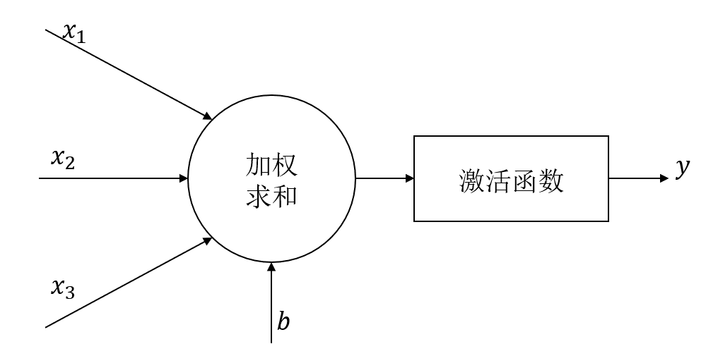
本方法略去了激活函数，直接将加权结果作为输出，加权公式为：
$y=x*w+b$
其中 $x$ 为 $1\times 4$ 矩阵， $y$ 为 $1\times 3$ 矩阵， $w$ 为 $4\times 3$ 的矩阵， $b$ 为 $1\times 3$ 矩阵

损失函数

用来描述预测值 $y$ 与真实标签 $y\underline{.}$ 的差距，本文方法使用均方误差来描述损失函数。
$MSE(y,y\underline{.})=\frac{\sum_{k=0}^n(y-y\underline{.})^2}{n}$

参数优化

为了找到一组参数 $w$ 和 $b$ 使损失函数最小，本文使用梯度下降法进行参数优化

梯度下降法：沿损失函数梯度下降的方向，寻找损失函数的最小值，得到最优参数的方法。

梯度下降法即对损失函数中的各个参量求偏导，得到的结果即为损失函数梯度下降的方向。公式如下
$w_{t+1}=w_t-lr\cdot \frac{\partial loss}{\partial w_t}\\ b_{t+1}=b_t-lr\cdot \frac{\partial loss}{\partial b_t}\\ w_{t+1}\cdot x+b_{t+1}\to y$
其中 $lr$ 表示学习率，不同的学习率会对参数更新造成不同的影响，如学习率过小，会造成参数更新过慢；学习率过大，会造成损失函数震荡。

3、程序实现

完整程序如下：

# -*- coding: utf-8 -*-
"""
Created on Thu Apr  9 11:01:13 2020
"""
# 鸢尾花分类
import tensorflow as tf
import numpy as np
from matplotlib import pyplot as plt


# 读入数据集
from sklearn.datasets import load_iris
x_data = load_iris().data
y_data = load_iris().target

# 打乱数据集
np.random.seed(116)
np.random.shuffle(x_data)
np.random.seed(116)
np.random.shuffle(y_data)

# 选择倒数第30之前的数据作为训练集
x_train = x_data[:-30]
y_train = y_data[:-30]
# 选择倒数第30之后的数据作为测试集
x_test  = x_data[-30:]
y_test  = y_data[-30:]

x_train = tf.cast(x_train, tf.float32)
x_test = tf.cast(x_test, tf.float32)

# 分批处理
train_db = tf.data.Dataset.from_tensor_slices((x_train, y_train)).batch(32)
test_db = tf.data.Dataset.from_tensor_slices((x_test, y_test)).batch(32)

# 随机初始化待更新的参数
w1 = tf.Variable(tf.random.truncated_normal([4, 3], stddev=0.1))
b1 = tf.Variable(tf.random.truncated_normal([3], stddev=0.1))

lr = 0.2 # 学习率/步长
epoch = 300 # 迭代总次数
loss_all = 0 # 每次迭代的损失
loss_list = [] # 存储每一次迭代的损失
acc_list = [] # 存储每一次迭代结果的准确率
for epoch in range(epoch):
    # 训练 
    # 更新权重
    for step, (x_train, y_train) in enumerate(train_db):
        with tf.GradientTape() as tape:
            # 前向传播得到当前权值下的推理结果 y = x * w1 + b1
            y = tf.matmul(x_train, w1) + b1;
            # 使用softmax将推理结果转换到[0, 1]之间
            y = tf.nn.softmax(y)
            # 将标签转换为独热码，即0:0 0 1, 1:0 1 0, 2:1 0 0
            y_ = tf.one_hot(y_train, depth=3)
            # 求均方误差
            loss = tf.reduce_mean(tf.square(y_ - y))
            loss_all += loss.numpy()
        # 分别对损失函数的w1、b1求偏导
        grads = tape.gradient(loss, [w1, b1])
        
        # 更新w1、b1 w1 = w1 - lr * w1_grad  b1 = b1 - lr * b1_grad
        w1.assign_sub(lr * grads[0])
        b1.assign_sub(lr * grads[1])
    # 打印此次迭代的损失
    print("Ecoph:{}, Loss:{}".format(epoch, loss_all / 4))
    loss_list.append(loss_all / 4)
    loss_all = 0
    
    # 测试
    # 计算此次迭代结果的正确率
    # 在真实训练时可以略过，这里只是为了画出正确率曲线
    total_correct, total_number = 0, 0
    for x_test, y_test in test_db:
        # 前向传播得到当前权值下的推理结果 y = x * w1 + b1
        y = tf.matmul(x_test, w1) + b1
        # 使用softmax将预测结果转换到[0, 1]之间
        y = tf.nn.softmax(y)
        # 找到最大值的索引
        pred = tf.argmax(y, axis=1)
        pred = tf.cast(pred, dtype=y_test.dtype)
        # 将预测结果与真实标签对比
        correct = tf.cast(tf.equal(pred, y_test), dtype=tf.int32)
        correct = tf.reduce_sum(correct)
        total_correct += int(correct)
        total_number += x_test.shape[0]
    acc = total_correct / total_number
    acc_list.append(acc)
    print("Acc:", acc)
    print("-------------------")
    
# 画出损失函数曲线
plt.plot(loss_list)
plt.title("Loss Curve")
plt.xlabel("Epoch")
plt.ylabel("Loss")
plt.show()
# 画出正确率曲线
plt.plot(acc_list)
plt.title("Acc Curve")
plt.xlabel("Epoch")
plt.ylabel("Acc")
plt.show()

4、运行结果

损失函数曲线如下，可以看到损失函数随着迭代次数的增加逐渐减小
正确率曲线

如有谬误，敬请指正！