TensorFlow实战--使用神经网络来实现对鸢尾花数据集的分类

利用单层神经网络实现对鸢尾花数据集的分类

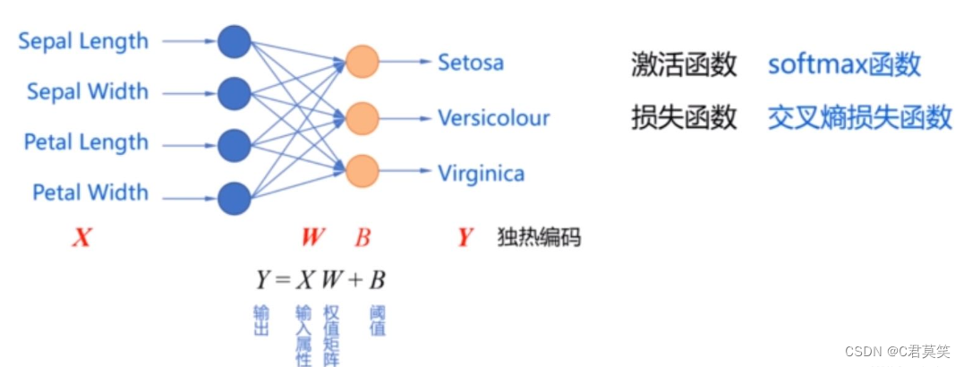
使用没有隐含层的单层前馈型神经网络来实现对鸢尾花的分类

import pandas as pd
import numpy as np
import tensorflow as tf
tf.enable_eager_execution() # 关键
import matplotlib.pyplot as plt

plt.rcParams['font.sans-serif'] = "SimHei"
plt.rcParams['axes.unicode_minus'] = False

# 目标：使用花萼长度、花萼宽度、花瓣长度、花瓣宽度四种属性将三种鸢尾花区分开

# 第一步：加载数据集
TRAIN_URL = "http://download.tensorflow.org/data/iris_training.csv"
train_path = tf.keras.utils.get_file(TRAIN_URL.split('/')[-1], TRAIN_URL)
df_iris_train = pd.read_csv(train_path, header=0)  # 表示第一行数据作为列标题

TEST_URL = "http://download.tensorflow.org/data/iris_test.csv"
test_path = tf.keras.utils.get_file(TEST_URL.split('/')[-1], TEST_URL)
df_iris_test = pd.read_csv(test_path, header=0)

# 第二步：数据处理
# 2.1 转化为NumPy数组
iris_train = np.array(df_iris_train)  # 将二维数据表转换为 Numpy 数组, (120, 5), iris的训练集中有120条样本,
iris_test = np.array(df_iris_test)  # 将二维数据表转换为 Numpy 数组, (30, 5), iris的测试集中有30条样本,

# 2.2 提取属性和标签
train_x = iris_train[:, 0:4]  # 取出鸢尾花训练数据集中属性列
train_y = iris_train[:, 4]  # 取出最后一列作为标签值, (120,)

test_x = iris_test[:, 0:4]  # 取出鸢尾花训练数据集中属性列
test_y = iris_test[:, 4]  # 取出最后一列作为标签值, (30, )

# 2.3 数据归一化
# 可以看出这两个属性的尺寸相同,因此不需要进行归一化,可以直接对其进行中心化处理
# 对每个属性进行中心化, 也就是按列中心化, 所以使用下面这种方式
train_x = train_x - np.mean(train_x, axis=0)
test_x = test_x - np.mean(test_x, axis=0)
# 此时样本点的横坐标和纵坐标的均值都是0

# 鸢尾花数据集中的属性值和标签值都是64位的浮点数
print(train_x.dtype)  # float64
print(train_y.dtype)  # float64

# 2.4 生成多元模型的属性矩阵和标签列向量
X_train = tf.cast(train_x, tf.float32)
# 创建张量函数tf.constant()
Y_train = tf.one_hot(tf.constant(train_y, dtype=tf.int32), 3)  # 将标签值转换为独热编码的形式
print(X_train.shape)  # (120, 4)
print(Y_train.shape)  # (120, 3)

X_test = tf.cast(test_x, tf.float32)
# 创建张量函数tf.constant()
Y_test = tf.one_hot(tf.constant(test_y, dtype=tf.int32), 3)  # 将标签值转换为独热编码的形式
print(X_test.shape)  # (30, 4)
print(Y_test.shape)  # (30, 3)

# 第三步：设置超参数和显示间隔
learn_rate = 0.2
itar = 500

display_step = 100

# 第四步：设置模型参数初始值
np.random.seed(612)
# 这里的W是一个(4, 3) 的矩阵
W = tf.Variable(np.random.randn(4, 3), dtype=tf.float32)
# 这里的B是一个(3, ) 的一维张量, 初始化为0
B = tf.Variable(np.zeros([3]), dtype=tf.float32)

# 第五步：训练模型
cross_train = []  # 列表cross_train用来保存每一次迭代的交叉熵损失
acc_train = []  # 用来存放训练集的分类准确率

cross_test = []  # 列表cross_test用来保存每一次迭代的交叉熵损失
acc_test = []  # 用来存放测试集的分类准确率

for i in range(0, itar + 1):

    with tf.GradientTape() as tape:

        # softmax 函数
        # X - (120, 4), W - (4, 3) , 所以 Pred_train - (120, 3), 是每个样本的预测概率
        Pred_train = tf.nn.softmax(tf.matmul(X_train, W) + B)
        # 计算训练集的平均交叉熵损失函数
        Loss_train = tf.reduce_mean(tf.keras.losses.categorical_crossentropy(y_true=Y_train, y_pred=Pred_train))

    Pred_test = tf.nn.softmax(tf.matmul(X_test, W) + B)
    # 计算测试集的平均交叉熵损失函数
    Loss_test = tf.reduce_mean(tf.keras.losses.categorical_crossentropy(y_true=Y_test, y_pred=Pred_test))

    # 计算准确率函数 -- 因为不需要对其进行求导运算, 因此也可以把这条语句写在 with 语句的外面
    Accuarcy_train = tf.reduce_mean(tf.cast(tf.equal(tf.argmax(Pred_train.numpy(), axis=1), train_y), tf.float32))
    Accuarcy_test = tf.reduce_mean(tf.cast(tf.equal(tf.argmax(Pred_test.numpy(), axis=1), test_y), tf.float32))

    # 记录每一次迭代的交叉熵损失和准确率
    cross_train.append(Loss_train)
    cross_test.append(Loss_test)
    acc_train.append(Accuarcy_train)
    acc_test.append(Accuarcy_test)

    # 对交叉熵损失函数 W 和 B 求偏导
    grads = tape.gradient(Loss_train, [W, B])
    # 函数assign_sub的作用是实现 Variable 变量的减法赋值
    # 更新模型参数 W
    W.assign_sub(learn_rate * grads[0])  # grads[0] 是 dL_dw, 形状为(4,3)
    # 更新模型偏置项参数 B
    B.assign_sub(learn_rate * grads[1])  # grads[1] 是 dL_db, 形状为(3, )

    if i % display_step == 0:
        print("i: %i, TrainLoss: %f, TrainAccuracy: %f, TestLoss: %f, TestAccuracy: %f"
              % (i, Loss_train, Accuarcy_train, Loss_test, Accuarcy_test))

"""
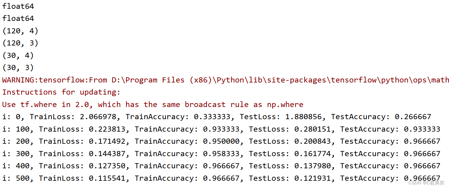
i: 0, TrainLoss: 2.066978, TrainAccuracy: 0.333333, TestLoss: 1.880855, TestAccuracy: 0.266667
i: 100, TrainLoss: 0.223813, TrainAccuracy: 0.933333, TestLoss: 0.280151, TestAccuracy: 0.933333
i: 200, TrainLoss: 0.171492, TrainAccuracy: 0.950000, TestLoss: 0.200843, TestAccuracy: 0.966667
i: 300, TrainLoss: 0.144387, TrainAccuracy: 0.958333, TestLoss: 0.161774, TestAccuracy: 0.966667
i: 400, TrainLoss: 0.127350, TrainAccuracy: 0.966667, TestLoss: 0.137980, TestAccuracy: 0.966667
i: 500, TrainLoss: 0.115541, TrainAccuracy: 0.966667, TestLoss: 0.121931, TestAccuracy: 0.966667
"""
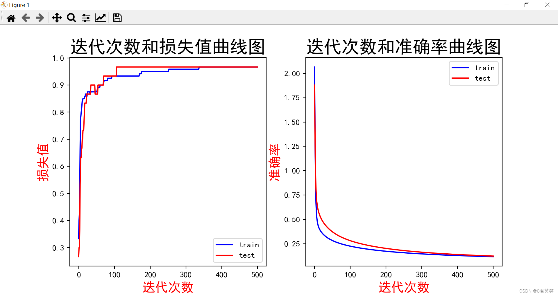
# 第六步：数据可视化
plt.figure(figsize=(12, 5))
plt.subplot(121)
plt.plot(acc_train, color="blue", label="train")
plt.plot(acc_test, color="red", label="test")
plt.title("迭代次数和损失值曲线图", fontsize=22)
plt.xlabel('迭代次数', color='r', fontsize=16)
plt.ylabel('损失值', color='r', fontsize=16)
plt.legend()

plt.subplot(122)
plt.plot(cross_train, color="blue", label="train")
plt.plot(cross_test, color="red", label="test")
plt.title("迭代次数和准确率曲线图", fontsize=22)
plt.xlabel('迭代次数', color='r', fontsize=16)
plt.ylabel('准确率', color='r', fontsize=16)
plt.legend()

plt.show()

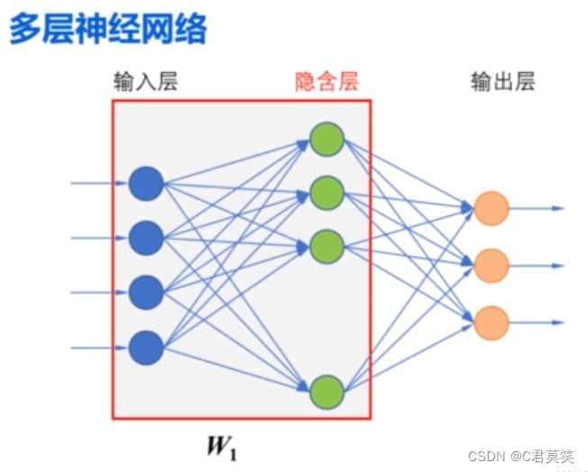
使用多层神经网络来实现对鸢尾花数据集的分类

第一层是输入层到隐含层，相应的权值矩阵为 W1 ，隐含层中的阈值是 B1 ，隐含层的输出是：

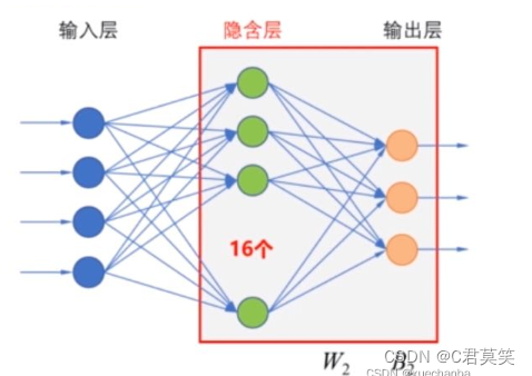
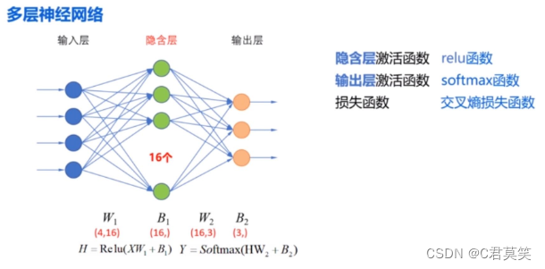
假设增加的隐含层中有 16 个神经元（结点），那么 B1 的形状就是 （16，），因为输入层中有四个结点，因此， W1 的形状是 （4，16），第二层是隐含层到输出层，从隐含层到输出层的权值矩阵为 W2 ，输出层中的阈值是 B2 ，因为输出层中有三个节点，所以B2 的形状是（3，），W2 的形状是（16，3）。

import pandas as pd
import numpy as np
import tensorflow as tf
tf.enable_eager_execution() # 关键
import matplotlib.pyplot as plt

plt.rcParams['font.sans-serif'] = "SimHei"
plt.rcParams['axes.unicode_minus'] = False

# 目标：使用花萼长度、花萼宽度、花瓣长度、花瓣宽度四种属性将三种鸢尾花区分开

# 第一步：加载数据集
TRAIN_URL = "http://download.tensorflow.org/data/iris_training.csv"
train_path = tf.keras.utils.get_file(TRAIN_URL.split('/')[-1], TRAIN_URL)
df_iris_train = pd.read_csv(train_path, header=0)  # 表示第一行数据作为列标题

TEST_URL = "http://download.tensorflow.org/data/iris_test.csv"
test_path = tf.keras.utils.get_file(TEST_URL.split('/')[-1], TEST_URL)
df_iris_test = pd.read_csv(test_path, header=0)

# 第二步：数据处理
# 2.1 转化为NumPy数组
iris_train = np.array(df_iris_train)  # 将二维数据表转换为 Numpy 数组, (120, 5), iris的训练集中有120条样本,
iris_test = np.array(df_iris_test)  # 将二维数据表转换为 Numpy 数组, (30, 5), iris的测试集中有30条样本,

# 2.2 提取属性和标签
train_x = iris_train[:, 0:4]  # 取出鸢尾花训练数据集中属性列
train_y = iris_train[:, 4]  # 取出最后一列作为标签值, (120,)

test_x = iris_test[:, 0:4]  # 取出鸢尾花训练数据集中属性列
test_y = iris_test[:, 4]  # 取出最后一列作为标签值, (30, )

# 2.3 数据归一化
# 可以看出这两个属性的尺寸相同,因此不需要进行归一化,可以直接对其进行中心化处理
# 对每个属性进行中心化, 也就是按列中心化, 所以使用下面这种方式
train_x = train_x - np.mean(train_x, axis=0)
test_x = test_x - np.mean(test_x, axis=0)
# 此时样本点的横坐标和纵坐标的均值都是0

# 2.4 生成多元模型的属性矩阵和标签列向量
X_train = tf.cast(train_x, tf.float32)
# 创建张量函数tf.constant()
Y_train = tf.one_hot(tf.constant(train_y, dtype=tf.int32), 3)  # 将标签值转换为独热编码的形式
print(X_train.shape)  # (120, 4)
print(Y_train.shape)  # (120, 3)

X_test = tf.cast(test_x, tf.float32)
# 创建张量函数tf.constant()
Y_test = tf.one_hot(tf.constant(test_y, dtype=tf.int32), 3)  # 将标签值转换为独热编码的形式
print(X_test.shape)  # (30, 4)
print(Y_test.shape)  # (30, 3)

# 第三步：设置超参数和显示间隔
learn_rate = 0.5
itar = 50

display_step = 10

# 第四步：设置模型参数初始值
np.random.seed(612)
# 隐含层
# 这里的 W1 是一个(4, 16) 的矩阵
W1 = tf.Variable(np.random.randn(4, 16), dtype=tf.float32)
# 这里的 B1 是一个(16, ) 的一维张量, 初始化为 0
B1 = tf.Variable(np.zeros([16]), dtype=tf.float32)
# 输出层
# 这里的 W2 是一个(16, 3) 的矩阵
W2 = tf.Variable(np.random.randn(16, 3), dtype=tf.float32)
# 这里的 B2 是一个(3, ) 的一维张量, 初始化为 0
B2 = tf.Variable(np.zeros([3]), dtype=tf.float32)

# 第五步：训练模型
cross_train = []  # 列表cross_train用来保存每一次迭代的交叉熵损失
acc_train = []  # 用来存放训练集的分类准确率

cross_test = []  # 列表cross_test用来保存每一次迭代的交叉熵损失
acc_test = []  # 用来存放测试集的分类准确率

for i in range(0, itar + 1):

    with tf.GradientTape() as tape:

        # 5.1：定义网络结构
        # H = X*W1 + B1
        Hidden_train = tf.nn.relu(tf.matmul(X_train, W1) + B1)
        # Y = H*W2 + B2
        Pred_train = tf.nn.softmax(tf.matmul(Hidden_train, W2) + B2)
        # 计算训练集的平均交叉熵损失函数
        Loss_train = tf.reduce_mean(tf.keras.losses.categorical_crossentropy(y_true=Y_train, y_pred=Pred_train))

        # H = X*W1 + B1
        Hidden_test = tf.nn.relu(tf.matmul(X_test, W1) + B1)
        # Y = H*W2 + B2
        Pred_test = tf.nn.softmax(tf.matmul(Hidden_test, W2) + B2)
        # 计算测试集的平均交叉熵损失函数
        Loss_test = tf.reduce_mean(tf.keras.losses.categorical_crossentropy(y_true=Y_test, y_pred=Pred_test))

    # 计算准确率函数 -- 因为不需要对其进行求导运算, 因此也可以把这条语句写在 with 语句的外面
    Accuarcy_train = tf.reduce_mean(tf.cast(tf.equal(tf.argmax(Pred_train.numpy(), axis=1), train_y), tf.float32))
    Accuarcy_test = tf.reduce_mean(tf.cast(tf.equal(tf.argmax(Pred_test.numpy(), axis=1), test_y), tf.float32))

    # 记录每一次迭代的交叉熵损失和准确率
    cross_train.append(Loss_train)
    cross_test.append(Loss_test)
    acc_train.append(Accuarcy_train)
    acc_test.append(Accuarcy_test)

    # 对交叉熵损失函数 W 和 B 求偏导
    grads = tape.gradient(Loss_train, [W1, B1, W2, B2])
    # 函数assign_sub的作用是实现 Variable 变量的减法赋值
    # 更新模型参数 W1
    W1.assign_sub(learn_rate * grads[0])  # grads[0] 是 dL_dw1, 形状为(4, 16)
    # 更新模型偏置项参数 B1
    B1.assign_sub(learn_rate * grads[1])  # grads[1] 是 dL_db1, 形状为(16, )
    # 更新模型参数 W2
    W2.assign_sub(learn_rate * grads[2])  # grads[0] 是 dL_dw2, 形状为(16, 3)
    # 更新模型偏置项参数 B2
    B2.assign_sub(learn_rate * grads[3])  # grads[1] 是 dL_db2, 形状为(3, )

    if i % display_step == 0:
        print("i: %i, TrainLoss: %f, TrainAccuracy: %f, TestLoss: %f, TestAccuracy: %f"
              % (i, Loss_train, Accuarcy_train, Loss_test, Accuarcy_test))

"""
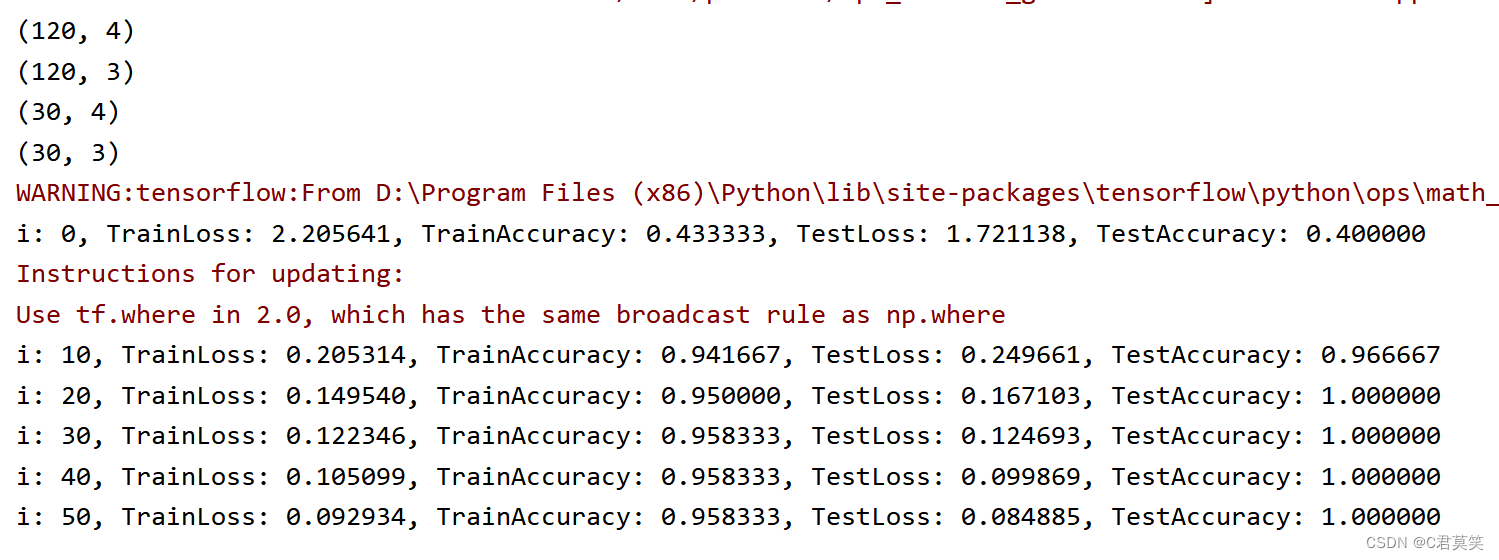
i: 0, TrainLoss: 2.205641, TrainAccuracy: 0.433333, TestLoss: 1.721138, TestAccuracy: 0.400000
i: 10, TrainLoss: 0.205314, TrainAccuracy: 0.941667, TestLoss: 0.249661, TestAccuracy: 0.966667
i: 20, TrainLoss: 0.149540, TrainAccuracy: 0.950000, TestLoss: 0.167103, TestAccuracy: 1.000000
i: 30, TrainLoss: 0.122346, TrainAccuracy: 0.958333, TestLoss: 0.124693, TestAccuracy: 1.000000
i: 40, TrainLoss: 0.105099, TrainAccuracy: 0.958333, TestLoss: 0.099869, TestAccuracy: 1.000000
i: 50, TrainLoss: 0.092934, TrainAccuracy: 0.958333, TestLoss: 0.084885, TestAccuracy: 1.000000
"""
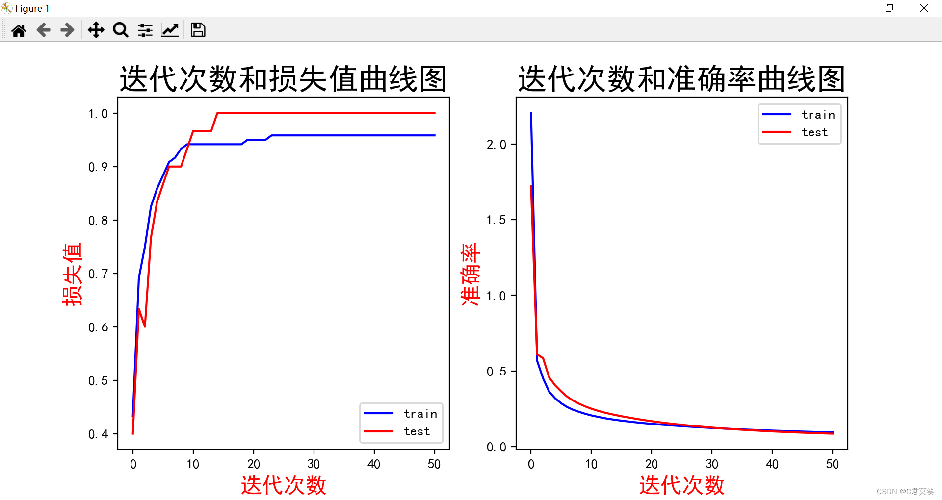
# 第六步：数据可视化
plt.figure(figsize=(12, 5))
plt.subplot(121)
plt.plot(acc_train, color="blue", label="train")
plt.plot(acc_test, color="red", label="test")
plt.title("迭代次数和损失值曲线图", fontsize=22)
plt.xlabel('迭代次数', color='r', fontsize=16)
plt.ylabel('损失值', color='r', fontsize=16)
plt.legend()

plt.subplot(122)
plt.plot(cross_train, color="blue", label="train")
plt.plot(cross_test, color="red", label="test")
plt.title("迭代次数和准确率曲线图", fontsize=22)
plt.xlabel('迭代次数', color='r', fontsize=16)
plt.ylabel('准确率', color='r', fontsize=16)
plt.legend()

plt.show()

对比单层神经网络和多层神经网络实现的对鸢尾花数据集的分类的效果。