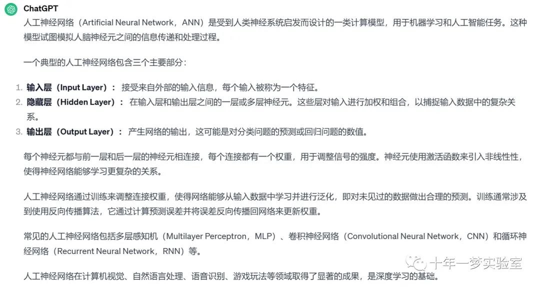
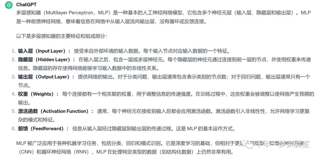
一、MLP 原理
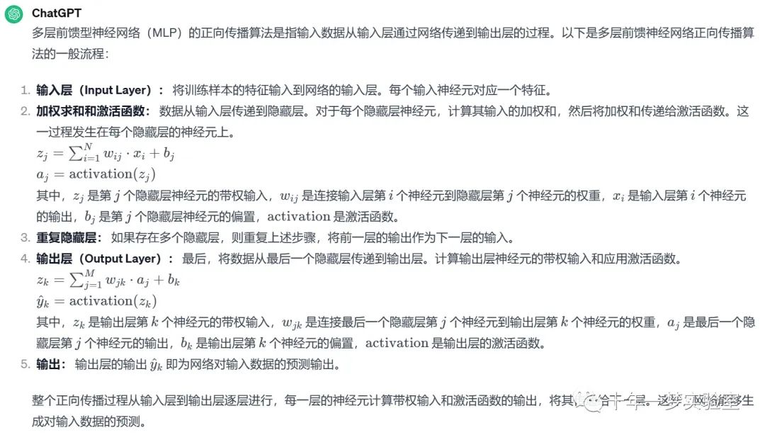
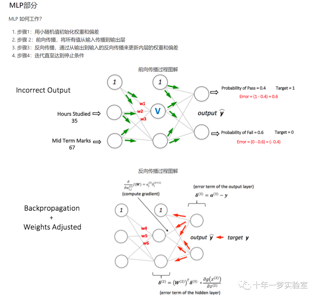
多层前馈型神经网络正向传播算法的流程
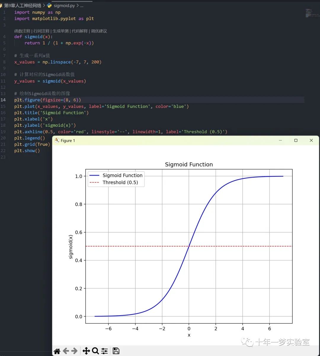
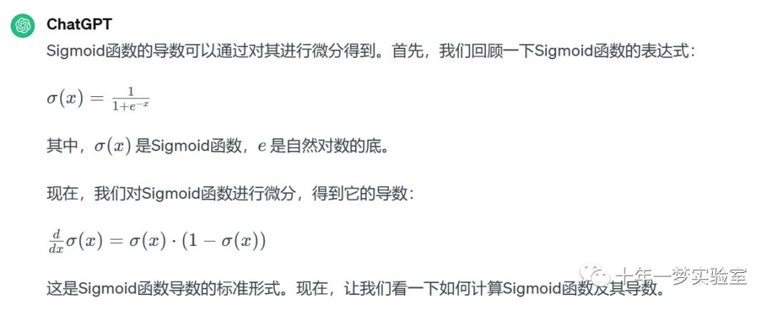
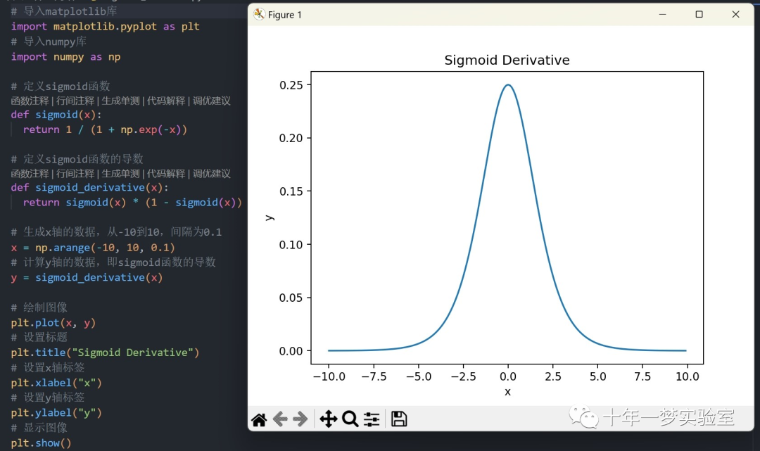
Sigmoid函数及其导数

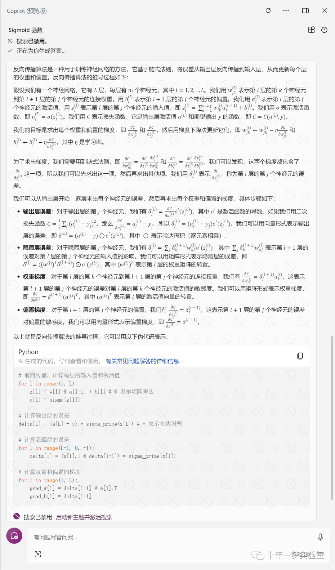
反向传播算法
二、示例-多层感知器(MLP)对鸢尾花数据集进行分类
2.1 多层感知器(MLP)的简单实现,主要用于解决鸢尾花数据集的分类问题。
以下是代码的主要步骤和功能:
1. 导入所需的库:导入了用于数据处理、可视化和神经网络的库。
2. 加载和检查数据集:使用 pandas 加载鸢尾花数据集,并进行简要的数据检查。
3. 数据清理过程:将数据集标签进行数字编码,将鸢尾花的三个类别分别编码为数字 0、1 和 2。
4. 将数据集分为训练集和测试集:将数据集分为训练集和测试集,并对数据进行随机排序。
5. MLP 部分:定义了一个 `MultiLayerPerceptron` 类,包含了 MLP 的初始化、权重初始化、激活函数和导数的定义等。
6. 定义反向传播过程算法:在 `Backpropagation_Algorithm` 函数中定义了 MLP 的反向传播算法,用于更新权重。
7. 定义用于绘制每个 epoch 误差值的函数:`show_err_graphic` 函数用于绘制每个 epoch 的误差值图。
8. 定义用于预测测试数据的 `predict` 函数。
9. 定义用于训练过程的 `fit` 函数:`fit` 函数用于训练 MLP 模型。
10. 使用训练数据训练 MLP 模型:使用给定的参数初始化 `MultiLayerPerceptron` 类,然后调用 `fit` 函数进行模型训练。
11. 使用 MLP 模型预测测试数据:使用训练好的 MLP 模型调用 `predict` 函数进行测试数据的预测。
12. 计算混淆矩阵和分类报告:计算混淆矩阵和打印每个类别的精确度、召回率和 F1 分数。
这个代码实现了一个简单的 MLP 模型,并在鸢尾花数据集上进行了训练和测试。请注意,这只是一个基础的实现,实际应用中可能需要进行更多的调优和改进。
数据集简要信息
鸢尾花数据集,也称为 Fisher’s Iris,是由英国统计学家兼生物学家 Ronald Fisher 提出的数据集,对科学做出了多项贡献。 罗纳德·费希尔 (Ronald Fisher) 因其论文《在分类问题中使用多重测量作为线性判别分析的示例》而闻名于世。 Ronald Fisher 在这篇论文中介绍了鸢尾花数据集。
The Iris Flower Dataset, also called Fisher’s Iris, is a dataset introduced by Ronald Fisher, a British statistician, and biologist, with several contributions to science. Ronald Fisher has well known worldwide for his paper The use of multiple measurements in taxonomic problems as an example of linear discriminant analysis. It was in this paper that Ronald Fisher introduced the Iris flower dataset.
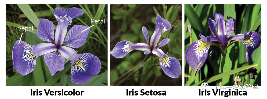
鸢尾花数据库由分布在三种不同鸢尾属植物中的 50 个样本组成。 每个样本都有特定的特征,这使得它们可以分为三类:山鸢尾、维吉尼亚鸢尾和杂色鸢尾。
The iris database consists of 50 samples distributed among three different species of iris. Each of these samples has specific characteristics, which allows them to be classified into three categories: Iris Setosa, Iris Virginica, and Iris versicolor.
# 导入所需的库
import os # 用于文件操作
from matplotlib import pyplot as plt # 用于数据可视化
import pandas as pd # 用于加载和处理原始数据集
import numpy as np # 用于数值计算
import random # 用于生成随机数
from pandas.plotting import scatter_matrix # 用于绘制散点图矩阵
加载和检查数据集
# 加载和检查数据集
# 设置工作目录并加载数据
os.chdir('./mlp-from-scratch-master/iris_dataset')


# 使用pandas读取和检查数据集
iris_dataset = pd.read_csv('iris.csv')
iris_dataset.head() # 查看数据集的前几行
iris_dataset[50:56] # 查看数据集的中间几行
iris_dataset.tail() # 查看数据集的后几行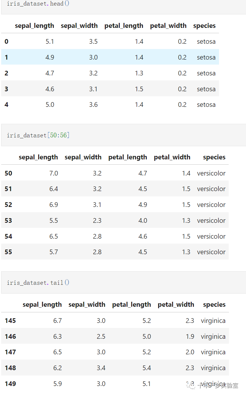
可视化原始数据集
# 可视化原始数据集
scatter_matrix(iris_dataset, alpha=0.5, figsize=(20, 20)) # 绘制数据集的散点图矩阵
#plt.show() # 显示图像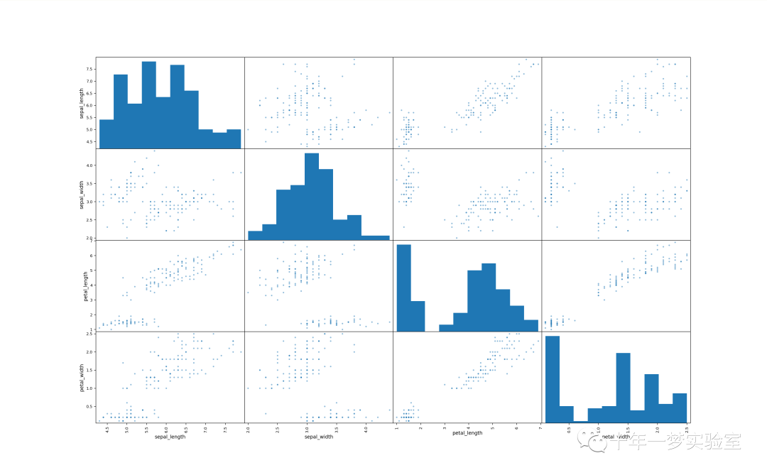
iris_dataset.plot(subplots=True, figsize=(10, 10), sharex=False, sharey=False) # 绘制数据集的折线图
#plt.show() # 显示图像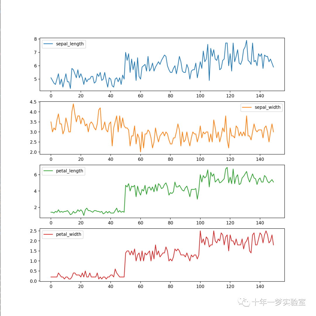
数据清洗流程
# 对数据集的标签进行数字编码,0: Iris-Setosa, 1: Iris-Versicolor, 2: Iris-Virginica
print('[INFO] create numeric classes for species (0,1,2) ...')


iris_dataset.loc[iris_dataset['species']=='setosa','species']=0 # 将setosa替换为0
iris_dataset.loc[iris_dataset['species']=='versicolor','species']=1 # 将versicolor替换为1
iris_dataset.loc[iris_dataset['species']=='virginica','species'] = 2 # 将virginica替换为2


iris_label = np.array(iris_dataset['species']) # 将标签转换为numpy数组
iris_data = np.array(iris_dataset[['sepal_length','sepal_width',
                                'petal_length', 'petal_width']]) # 将特征转换为numpy数组
划分数据集为训练集和测试集
# 划分数据集为训练集和测试集
random.seed(123) # 设置随机数种子


def separate_data(): # 定义一个函数,用于划分数据集
    A = iris_dataset[0:40] # 取每个类别的前40个样本作为训练集
    tA = iris_dataset[40:50] # 取每个类别的后10个样本作为测试集
    B = iris_dataset[50:90]
    tB = iris_dataset[90:100]
    C = iris_dataset[100:140]
    tC = iris_dataset[140:150]
    train = np.concatenate((A,B,C)) # 将不同类别的训练集拼接起来
    test =  np.concatenate((tA,tB,tC)) # 将不同类别的测试集拼接起来
    return train,test # 返回训练集和测试集


print('[INFO] separate data to train data and test data')
iris_dataset = np.column_stack((iris_data,iris_label.T)) # 将特征和标签拼接起来
iris_dataset = list(iris_dataset) # 将数据集转换为列表
random.shuffle(iris_dataset) # 打乱数据集的顺序
Filetrain, Filetest = separate_data() # 调用划分数据集的函数


#[i[:4] for i in Filetrain]:这是一个列表推导式,它遍历Filetrain列表中的每个元素i,
# 对于每个元素i,它取i的前四个值(即i[:4]),并将这四个值作为一个子列表添加到新的列表中。
# 这样,新的列表就包含了Filetrain中每个样本的四个特征,而不包括标签。
train_X = np.array([i[:4] for i in Filetrain]).astype('float') # 提取训练集的特征,并转换为浮点数
train_y = np.array([i[4] for i in Filetrain]).astype('float') # 提取训练集的标签,并转换为浮点数
test_X = np.array([i[:4] for i in Filetest]).astype('float') # 提取测试集的特征,并转换为浮点数
test_y = np.array([i[4] for i in Filetest]).astype('float') # 提取测试集的标签,并转换为浮点数
print('train data shape: ', train_X.shape) # 打印训练集的形状
print('test data shape: ', test_X.shape) # 打印测试集的形状
print('train label shape: ', train_y.shape) # 打印训练集的标签的形状
print('test label shape: ', test_y.shape) # 打印测试集的标签的形状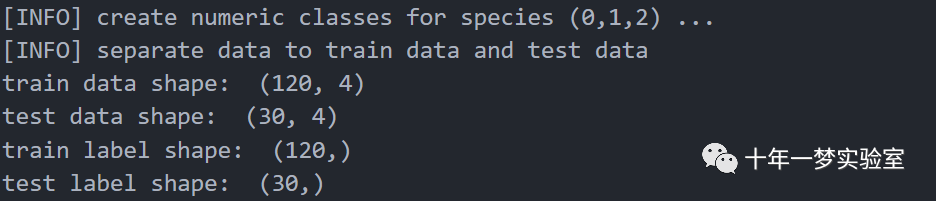
定义多层感知器(MLP)类对象
# 定义多层感知器(MLP)类对象
class MultiLayerPerceptron:
def __init__(self, params=None): # 定义初始化方法,接受一个参数params
# 如果params为空,则使用默认的MLP层参数
if (params == None):
self.inputLayer = 4 # 输入层的节点数
self.hiddenLayer = 5 # 隐藏层的节点数
self.outputLayer = 3 # 输出层的节点数
self.learningRate = 0.005 # 学习率
self.max_epochs = 600 # 最大迭代次数
self.BiasHiddenValue = -1 # 隐藏层的偏置值
self.BiasOutputValue = -1 # 输出层的偏置值
self.activation = self.activation['sigmoid'] # 激活函数
self.deriv = self.deriv['sigmoid'] # 激活函数的导数
else:
# 如果params不为空,则使用params指定的MLP层参数
self.inputLayer = params['InputLayer']
self.hiddenLayer = params['HiddenLayer']
self.OutputLayer = params['OutputLayer']
self.learningRate = params['LearningRate']
self.max_epochs = params['Epochs']
self.BiasHiddenValue = params['BiasHiddenValue']
self.BiasOutputValue = params['BiasOutputValue']
self.activation = self.activation[params['ActivationFunction']]
self.deriv = self.deriv[params['ActivationFunction']]
# 初始化权重和偏置值
self.WEIGHT_hidden = self.starting_weights(self.hiddenLayer, self.inputLayer) # 隐藏层的权重矩阵
self.WEIGHT_output = self.starting_weights(self.OutputLayer, self.hiddenLayer) # 输出层的权重矩阵
self.BIAS_hidden = np.array([self.BiasHiddenValue for i in range(self.hiddenLayer)]) # 隐藏层的偏置向量
self.BIAS_output = np.array([self.BiasOutputValue for i in range(self.OutputLayer)]) # 输出层的偏置向量
self.classes_number = 3 # 类别数
pass
def starting_weights(self, x, y): # 定义一个函数,用于生成初始的权重矩阵
return [[2 * random.random() - 1 for i in range(x)] for j in range(y)] # 生成一个x行y列的随机数矩阵,范围在-1到1之间
# 定义激活函数和导数函数,根据数学公式实现
activation = {
'sigmoid': (lambda x: 1/(1 + np.exp(-x * 1.0))), # sigmoid函数
'tanh': (lambda x: np.tanh(x)), # 双曲正切函数
'Relu': (lambda x: x*(x > 0)), # 线性整流函数
}
deriv = {
'sigmoid': (lambda x: x*(1-x)), # sigmoid函数的导数
'tanh': (lambda x: 1-x**2), # 双曲正切函数的导数
'Relu': (lambda x: 1 * (x>0)) # 线性整流函数的导数
}
# 定义反向传播算法的过程
def Backpropagation_Algorithm(self, x): # 定义一个函数,接受一个参数x,表示输入层的数据
DELTA_output = [] # 定义一个空列表,用于存储输出层的误差梯度
# 第一阶段 - 计算输出层的误差
ERROR_output = self.output - self.OUTPUT_L2 # 输出层的误差等于期望输出减去实际输出
DELTA_output = ((-1)*(ERROR_output) * self.deriv(self.OUTPUT_L2)) # 输出层的误差梯度等于误差乘以输出层的导数
arrayStore = [] # 定义一个空列表,用于存储中间结果
# 第二阶段 - 更新输出层和隐藏层的权重和偏置
for i in range(self.hiddenLayer): # 遍历隐藏层的每个节点
for j in range(self.OutputLayer): # 遍历输出层的每个节点
self.WEIGHT_output[i][j] -= (self.learningRate * (DELTA_output[j] * self.OUTPUT_L1[i])) # 更新输出层的权重,使用梯度下降法
self.BIAS_output[j] -= (self.learningRate * DELTA_output[j]) # 更新输出层的偏置,使用梯度下降法
# 第三阶段 - 计算隐藏层的误差
delta_hidden = np.matmul(self.WEIGHT_output, DELTA_output)* self.deriv(self.OUTPUT_L1) # 隐藏层的误差梯度等于输出层的权重矩阵乘以输出层的误差梯度,再乘以隐藏层的导数
# 第四阶段 - 更新隐藏层和输入层的权重和偏置
for i in range(self.OutputLayer): # 遍历输入层的每个节点
for j in range(self.hiddenLayer): # 遍历隐藏层的每个节点
self.WEIGHT_hidden[i][j] -= (self.learningRate * (delta_hidden[j] * x[i])) # 更新隐藏层的权重,使用梯度下降法
self.BIAS_hidden[j] -= (self.learningRate * delta_hidden[j]) # 更新隐藏层的偏置,使用梯度下降法
# 定义一个函数,用于绘制每个迭代的误差值
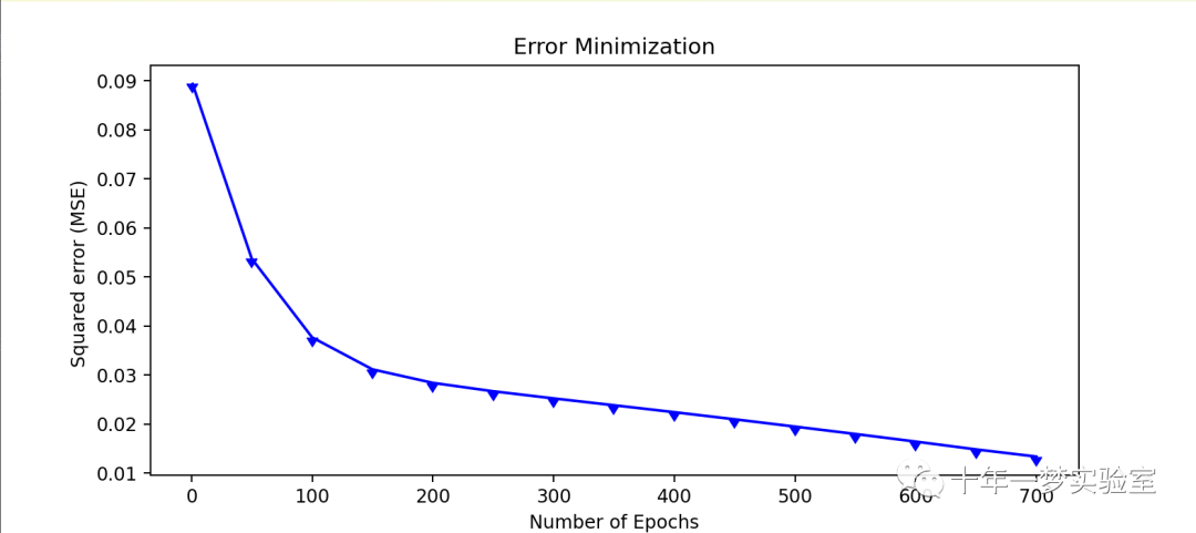
def show_err_graphic(self,v_error,v_epoch): # 定义一个函数,接受两个参数,分别是误差值和迭代次数的列表
plt.figure(figsize=(9,4)) # 创建一个图像对象,设置大小为9x4
plt.plot(v_epoch, v_error, "-",color="b", marker=11) # 绘制误差值随迭代次数的变化曲线,设置颜色和标记
plt.xlabel("Number of Epochs") # 设置x轴的标签
plt.ylabel("Squared error (MSE) ") # 设置y轴的标签
plt.title("Error Minimization") # 设置标题
plt.show() # 显示图像
# 定义用于预测测试数据的predict函数
def predict(self, X, y): # 定义一个函数,接受两个参数,分别是测试集的特征和标签
my_predictions = [] # 定义一个空列表,用于存储预测值
# 只进行前向传播
forward = np.matmul(X,self.WEIGHT_hidden) + self.BIAS_hidden # 计算输入层到隐藏层的线性组合,加上隐藏层的偏置
forward = np.matmul(forward, self.WEIGHT_output) + self.BIAS_output # 计算隐藏层到输出层的线性组合,加上输出层的偏置
for i in forward: # 遍历输出层的每个节点
my_predictions.append(max(enumerate(i), key=lambda x:x[1])[0]) # 将输出层的最大值对应的索引作为预测值
# 打印预测值
print(" Number of Sample | Class | Output | Hoped Output") # 打印表头
for i in range(len(my_predictions)): # 遍历每个样本
if(my_predictions[i] == 0): # 如果预测值为0,表示setosa类别
print("id:{} | Iris-Setosa | Output: {} | Hoped Output:{} ".format(i, my_predictions[i], y[i])) # 打印样本的id,类别,输出值和期望值
elif(my_predictions[i] == 1): # 如果预测值为1,表示versicolor类别
print("id:{} | Iris-Versicolour | Output: {} | Hoped Output:{} ".format(i, my_predictions[i], y[i])) # 打印样本的id,类别,输出值和期望值
elif(my_predictions[i] == 2): # 如果预测值为2,表示virginica类别
print("id:{} | Iris-Iris-Virginica | Output: {} | Hoped Output:{} ".format(i, my_predictions[i], y[i])) # 打印样本的id,类别,输出值和期望值
return my_predictions # 返回预测值列表
pass
# 定义用于训练过程的fit函数,使用训练数据
def fit(self, X, y): # 定义一个函数,接受两个参数,分别是训练集的特征和标签
count_epoch = 1 # 定义一个变量,用于记录迭代次数
total_error = 0 # 定义一个变量,用于记录总误差
n = len(X); # 定义一个变量,用于记录样本数
epoch_array = [] # 定义一个空列表,用于存储迭代次数
error_array = [] # 定义一个空列表,用于存储误差值
W0 = [] # 定义一个空列表,用于存储隐藏层的权重
W1 = [] # 定义一个空列表,用于存储输出层的权重
while(count_epoch <= self.max_epochs): # 当迭代次数小于等于最大迭代次数时,循环执行
for idx,inputs in enumerate(X): # 遍历训练集的每个样本,获取索引和输入
self.output = np.zeros(self.classes_number) # 初始化输出为零向量
# 阶段1 - (前向传播)
self.OUTPUT_L1 = self.activation((np.dot(inputs, self.WEIGHT_hidden) + self.BIAS_hidden.T)) # 计算输入层到隐藏层的线性组合,加上隐藏层的偏置,然后通过激活函数,得到隐藏层的输出
self.OUTPUT_L2 = self.activation((np.dot(self.OUTPUT_L1, self.WEIGHT_output) + self.BIAS_output.T)) # 计算隐藏层到输出层的线性组合,加上输出层的偏置,然后通过激活函数,得到输出层的输出
# 阶段2 - One-Hot-Encoding
if(y[idx] == 0): # 如果标签为0,表示setosa类别
self.output = np.array([1,0,0]) # 输出为[1,0,0],表示第一个类别的概率为1,其他为0
elif(y[idx] == 1): # 如果标签为1,表示versicolor类别
self.output = np.array([0,1,0]) # 输出为[0,1,0],表示第二个类别的概率为1,其他为0
elif(y[idx] == 2): # 如果标签为2,表示virginica类别
self.output = np.array([0,0,1]) # 输出为[0,0,1],表示第三个类别的概率为1,其他为0
square_error = 0 # 定义一个变量,用于记录平方误差
for i in range(self.OutputLayer): # 遍历输出层的每个节点
erro = (self.output[i] - self.OUTPUT_L2[i])**2 # 计算期望输出和实际输出的差的平方
square_error = (square_error + (0.05 * erro)) # 将平方误差乘以0.05,累加到总的平方误差中
total_error = total_error + square_error # 将平方误差累加到总误差中
# 阶段3 - (反向传播):更新权重
self.Backpropagation_Algorithm(inputs) # 调用反向传播算法的函数,传入输入作为参数
total_error = (total_error / n) # 计算平均误差
# 每个epoch打印一次误差值
if((count_epoch % 50 == 0)or(count_epoch == 1)): # 如果迭代次数是50的倍数或者1,打印当前的迭代次数和误差值
print("Epoch ", count_epoch, "- Total Error: ",total_error) # 打印迭代次数和误差值
error_array.append(total_error) # 将误差值添加到误差值列表中
epoch_array.append(count_epoch) # 将迭代次数添加到迭代次数列表中
W0.append(self.WEIGHT_hidden) # 将隐藏层的权重添加到隐藏层权重列表中
W1.append(self.WEIGHT_output) # 将输出层的权重添加到输出层权重列表中
count_epoch += 1 # 迭代次数加一
self.show_err_graphic(error_array,epoch_array) # 调用绘制误差值图像的函数,传入误差值列表和迭代次数列表
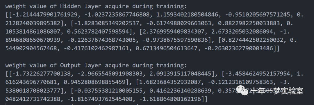
# 打印训练期间获取的隐藏层权重
print('') # 打印一个空行
print('weight value of Hidden layer acquire during training: ') # 打印提示信息
print(W0[0]) # 打印隐藏层权重列表的第一个元素,即初始的隐藏层权重
# 打印训练期间获取的输出层权重
print('') # 打印一个空行
print('weight value of Output layer acquire during training: ') # 打印提示信息
print(W1[0]) # 打印输出层权重列表的第一个元素,即初始的输出层权重
return self # 返回自身对象使用训练数据训练MLP模型
# 让我们尝试一下我们的MLP
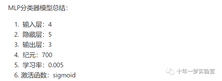
dictionary = {'InputLayer':4, 'HiddenLayer':5, 'OutputLayer':3,
'Epochs':700, 'LearningRate':0.005,'BiasHiddenValue':-1,
'BiasOutputValue':-1, 'ActivationFunction':'sigmoid'}
# 定义一个字典,包含MLP模型的参数,如输入层、隐藏层、输出层的神经元个数,训练轮数,学习率,偏置值,激活函数
Perceptron = MultiLayerPerceptron(dictionary)
# 创建一个MultiLayerPerceptron类的实例,传入字典作为参数
Perceptron.fit(train_X,train_y)
# 调用fit方法,使用训练数据集train_X和train_y训练MLP模型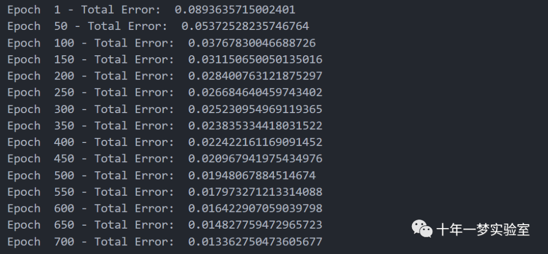
使用 MLP 模型预测测试数据
# 使用MLP模型预测测试数据
pred = Perceptron.predict(test_X,test_y)
# 调用predict方法,使用测试数据集test_X和test_y预测MLP模型的输出,返回一个列表pred,存储预测的类别


pred = np.array(pred)
# 将pred列表转换为numpy数组,方便后续计算


true = test_y.astype('int')
# 将test_y数组转换为整数类型,方便后续计算


def compute_confusion_matrix(true, pred):
    '''
    用numpy计算两个np.arrays的混淆矩阵
    结果与以下相同(计算时间相似):
    "from sklearn.metrics import confusion_matrix"
    但是,此函数避免了对sklearn的依赖。
    '''
    # 定义一个函数,计算真实值和预测值的混淆矩阵,不需要使用sklearn库


    K = len(np.unique(true)) # Number of classes
    # 计算类别的个数,赋值给K


    result = np.zeros((K, K))
    # 创建一个K*K的零矩阵,用于存储混淆矩阵的结果


    for i in range(len(true)):
        # 遍历真实值的每个元素
        result[true[i]][pred[i]] += 1
        # 根据真实值和预测值的对应关系,将结果矩阵的相应位置加一


    return result
    # 返回结果矩阵


conf_matrix = compute_confusion_matrix(true, pred)
# 调用compute_confusion_matrix函数,传入真实值和预测值,得到混淆矩阵,赋值给conf_matrix


print('Confussion matrix result: ')
# 打印混淆矩阵的结果


print(conf_matrix)
# 打印conf_matrix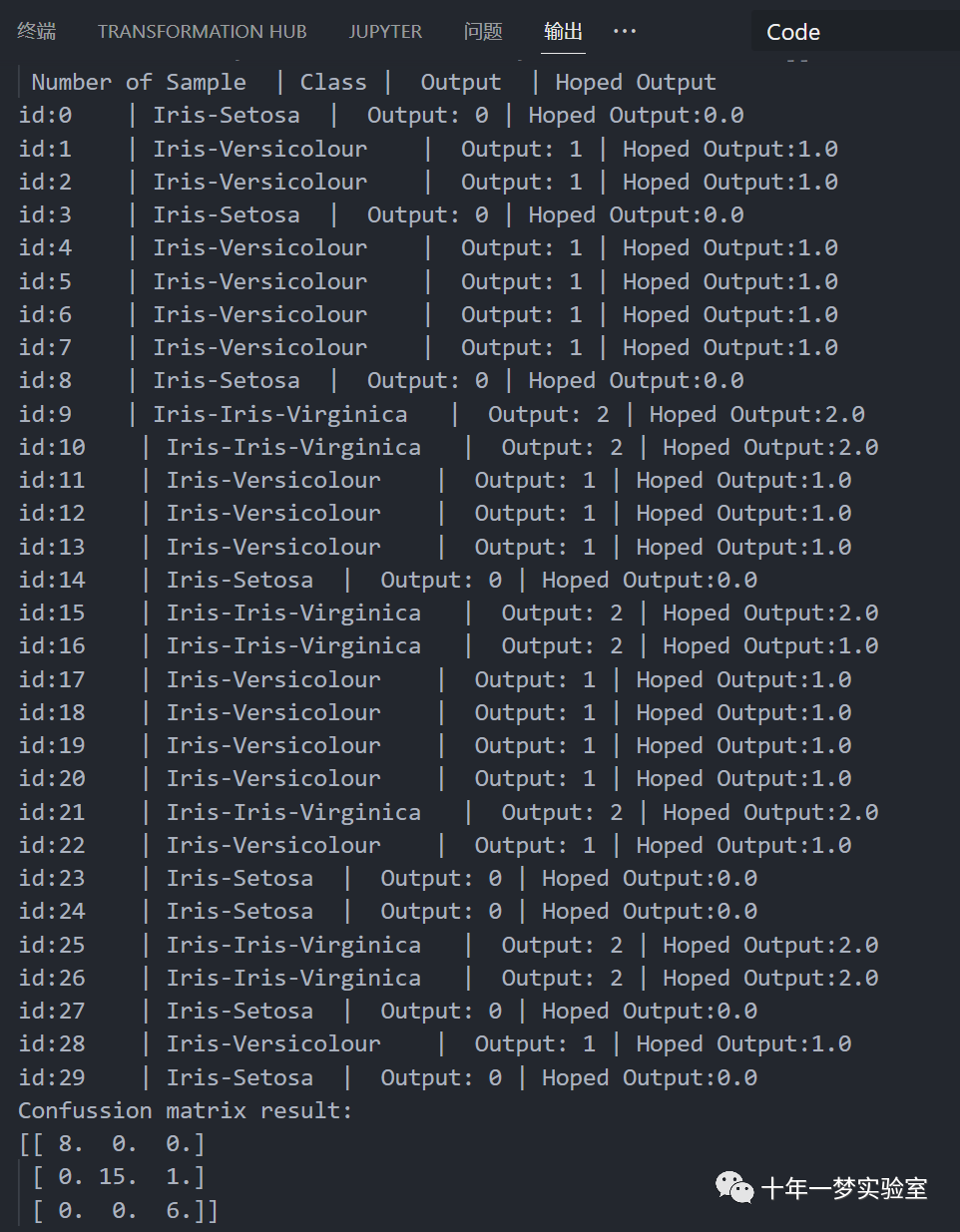
分类报告
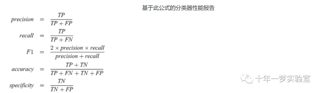
# 分类报告
classes = ['setosa    ', 'versicolor', 'virginica ']
# 定义一个列表,存储三个类别的名称


def accuracy_average(confusion_matrix):
    # 定义一个函数,计算混淆矩阵的平均准确率
    diagonal_sum = confusion_matrix.trace()
    # 计算混淆矩阵的对角线之和,即正确分类的个数
    sum_of_all_elements = confusion_matrix.sum()
    # 计算混淆矩阵的所有元素之和,即总的样本个数
    return diagonal_sum / sum_of_all_elements
    # 返回对角线之和除以所有元素之和,即平均准确率


def precision(label, confusion_matrix):
    # 定义一个函数,计算混淆矩阵的某个类别的精确度
    col = confusion_matrix[:, label]
    # 取混淆矩阵的第label列,即预测为该类别的个数
    return confusion_matrix[label, label] / col.sum()
    # 返回混淆矩阵的第label行第label列的元素,即正确预测为该类别的个数,除以第label列的元素之和,即精确度


def recall(label, confusion_matrix):
    # 定义一个函数,计算混淆矩阵的某个类别的召回率
    row = confusion_matrix[label, :]
    # 取混淆矩阵的第label行,即真实为该类别的个数
    return confusion_matrix[label, label] / row.sum()
    # 返回混淆矩阵的第label行第label列的元素,即正确预测为该类别的个数,除以第label行的元素之和,即召回率


def f1_score(label, confusion_matrix):
    # 定义一个函数,计算混淆矩阵的某个类别的F1分数
    num = precision(label, confusion_matrix) * recall(label, confusion_matrix)
    # 计算精确度和召回率的乘积,赋值给num
    denum = precision(label, confusion_matrix) + recall(label, confusion_matrix)
    # 计算精确度和召回率的和,赋值给denum
    return 2 * (num/denum)
    # 返回2乘以num除以denum,即F1分数


def precision_macro_average(confusion_matrix):
    # 定义一个函数,计算混淆矩阵的平均精确度
    rows, columns = confusion_matrix.shape
    # 获取混淆矩阵的行数和列数,赋值给rows和columns
    sum_of_precisions = 0
    # 初始化一个变量,用于存储所有类别的精确度之和
    for label in range(rows):
        # 遍历每个类别
        sum_of_precisions += precision(label, confusion_matrix)
        # 调用precision函数,计算该类别的精确度,累加到sum_of_precisions
    return sum_of_precisions / rows
    # 返回sum_of_precisions除以rows,即平均精确度


def recall_macro_average(confusion_matrix):
    # 定义一个函数,计算混淆矩阵的平均召回率
    rows, columns = confusion_matrix.shape
    # 获取混淆矩阵的行数和列数,赋值给rows和columns
    sum_of_recalls = 0
    # 初始化一个变量,用于存储所有类别的召回率之和
    for label in range(columns):
        # 遍历每个类别
        sum_of_recalls += recall(label, confusion_matrix)
        # 调用recall函数,计算该类别的召回率,累加到sum_of_recalls
    return sum_of_recalls / columns
    # 返回sum_of_recalls除以columns,即平均召回率


def f1_score_average(confusion_matrix):
    # 定义一个函数,计算混淆矩阵的平均F1分数
    num = precision_macro_average(confusion_matrix) * recall_macro_average(confusion_matrix)
    # 计算平均精确度和平均召回率的乘积,赋值给num
    denum = precision_macro_average(confusion_matrix) + recall_macro_average(confusion_matrix)
    # 计算平均精确度和平均召回率的和,赋值给denum
    return 2 * (num/denum)
    # 返回2乘以num除以denum,即平均F1分数


print("label      precision  recall  f1_score")
# 打印标签,精确度,召回率,F1分数的表头


for index in range(len(classes)):
    # 遍历每个类别
    print(f"{classes[index]} {precision(index, conf_matrix):9.3f} {recall(index, conf_matrix):6.3f}  {f1_score(index, conf_matrix):6.3f}")
    # 打印该类别的名称,精确度,召回率,F1分数的表头
print()
print('Average accuracy:  ', accuracy_average(conf_matrix))
print('Average precision: ', precision_macro_average(conf_matrix))
print('Average recall:    ', recall_macro_average(conf_matrix))
print('Average F1 score:  ', f1_score_average(conf_matrix))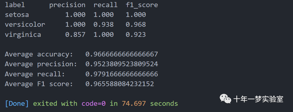
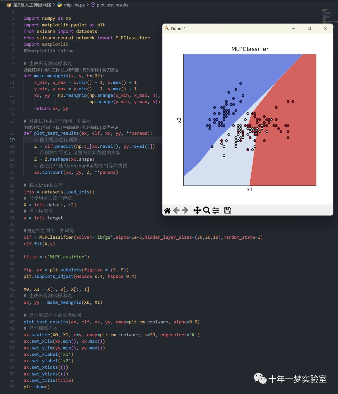
2.2 使用sklearn的MLP对iris数据集进行分类
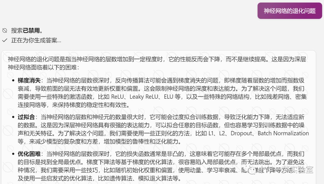
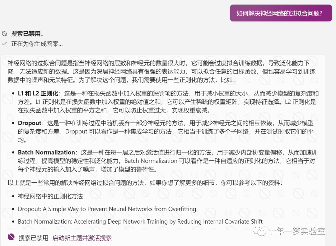
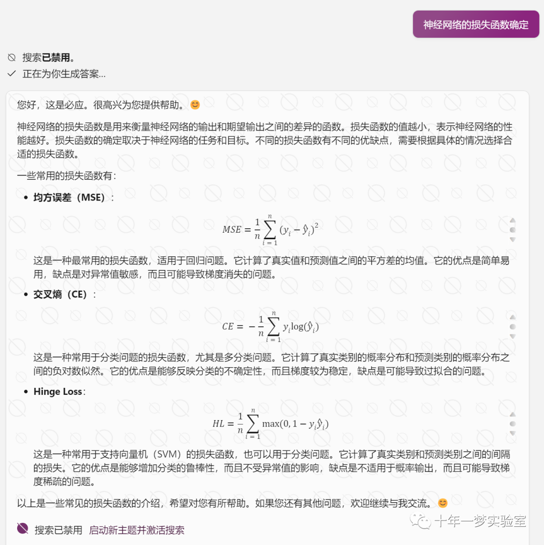
三、一些问题


四、实现细节


五、人工神经网络的应用
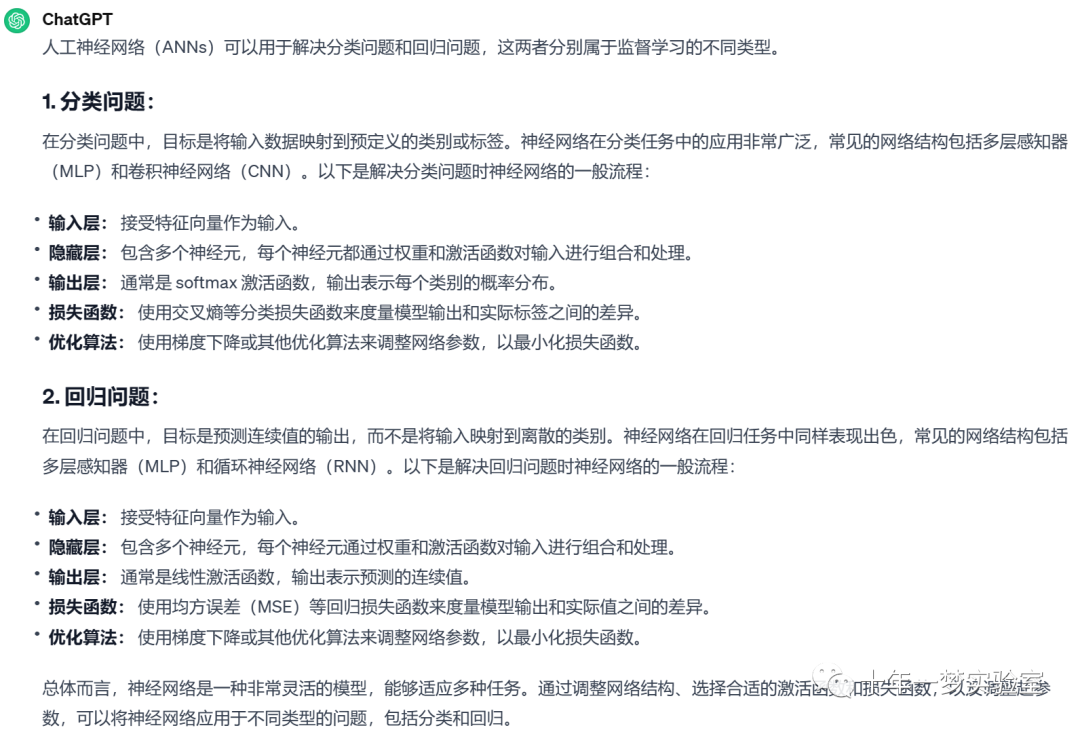
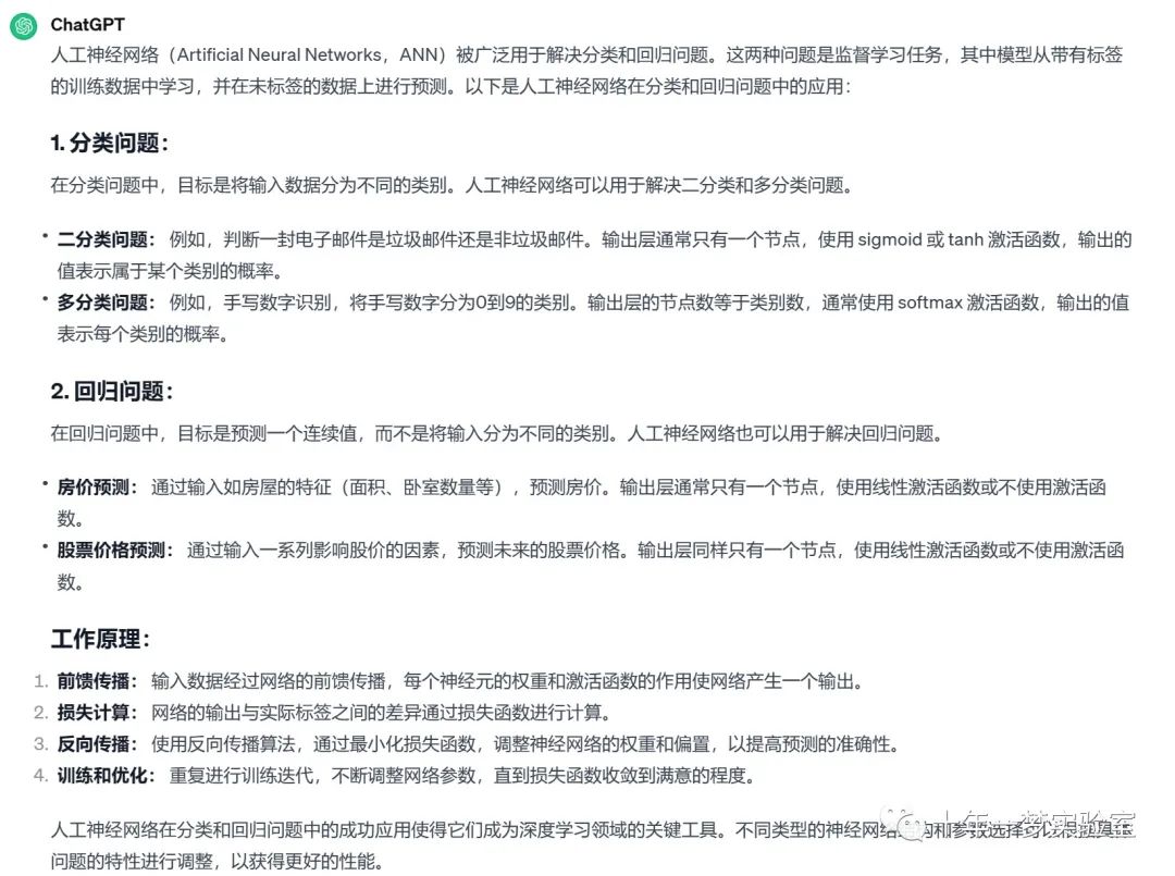
人工神经网络解决分类和回归问题
人工神经网络应用场景
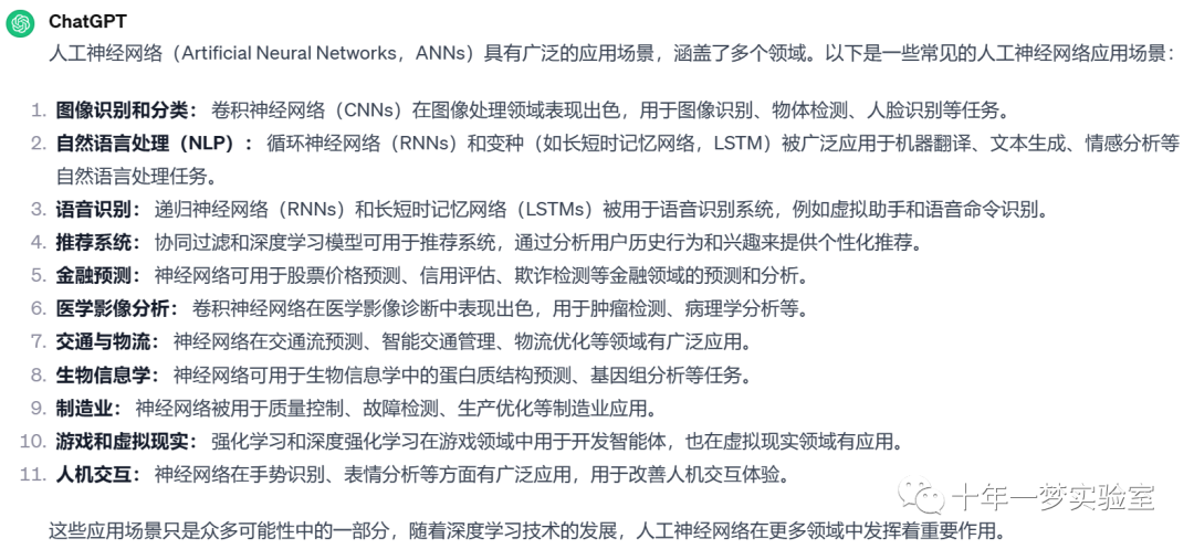
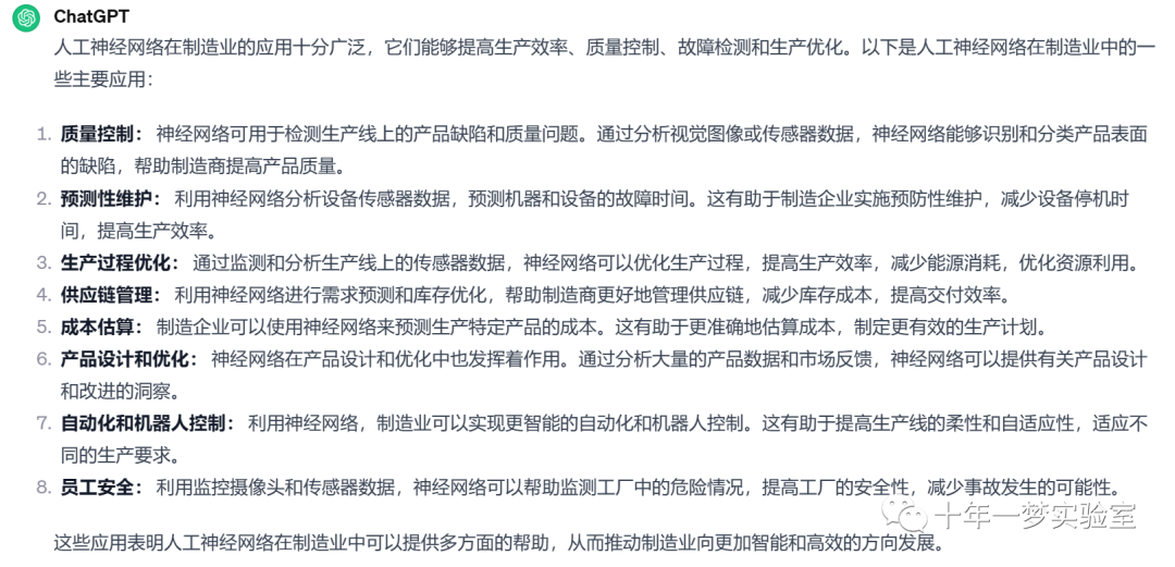
人工神经网络在制造业的应用
The End