抽点时间读经典AI论文之Learning representations by back-propagating errors

这篇论文讲述的是世界上第一篇反向传播算法,标题的意思是通过反向传播错误来学习表征

在读这篇论文时,我是带着这三个问题去读的:

1. 作者试图解决什么问题?
2. 这篇论文的关键元素是什么?
3. 论文中有什么内容可以"为你所用"?

于此同时,在讲解这篇论文时,我不会把论文全篇翻译出来,毕竟这样做毫无意义,我会把我个人觉得比较重要的部分摘出来,再结合我自己的认识,与大家分享

文章的一开头就给出了反向传播算法的原理:

The procedure repeatedly adjusts the weights of the connections in the network so as to minimize a measure of the dilference between the actual output vector of the net and the desired output vector.

该程序反复调整网络中连接的权重，以使网络的实际输出向量与期望输出向量之间的偏差最小化。

其实这个过程就是学习的过程,学习率就是用来调整权重的超参数,举个最简单的例子,输入一个数,如何让机器输出相反数呢?

不难知道,让这个数乘上-1即可,这个-1其实就是网络的权重,如果用数学表达,可以列出如下式子:

Y = A * X

• Y表示网络的输出,即相反数
• A表示权重,就是网络要学习的参数
• X表示输入网络的值,理论上可以是任意一个数

权重A在开始时可以随机设定一个数,比如1;如果学习率是0.1,那么需要至少20轮训练,才能让权重A从1变成-1

如果你看懂了这个过程,那么你可以看看我的这篇文章:

如何用Python教机器学会牛顿第二定律?

接着,论文提到了隐藏层,并描述了什么是隐藏层:

In perceptrons,there. are ‘feature analysers’ between the input and output that are not true hidden units because their input connections are fxed by hand, so their states are completely determined by the input vector: they do not learn representations.

简单来说,隐藏层是用来提取特征的。比如我输入了10个特征,隐藏层只定义5个特征,那么这就相当于把这10个小特征合并成了5个大特征,当然,你也可以根据需要,再把这5个特征合并

需要注意的是,这些特征都是人为定义好的,举个具体点的例子,在做人脸分析时输入图片的特征有肤色、发型、是单眼皮还是双眼皮、鼻子的大小等,然后将这些特征输入到人为定义好的隐藏层中,假如隐藏层定义的特征是好看、一般和不好看,那么输出的特征就会更抽象

也就是说,隐藏层的作用就是把具体的特征变得抽象

读到这里,不知道你有没有疑惑,隐藏层到底是怎么样把具体的特征变得抽象的?作者给出了两个公式:

• $x_j$ = $\sum_{i}y_iw_{ji}$     (1)

• $y_j$ = $\frac{1} {1 + e^{-x_j}}$        (2)

具体怎么用呢?这里举个例子:

假设有两个输入,分别是1,箭头上的数字代表权重,箭头的指向表示输出,下面我们来算一下第一个隐藏层的输入值 $x_1$ = 1 * 0.8 + 1 * 0.2 = 1

第二个隐藏层的输入也不难得到:
$x_2$ = 1 * 0.4 + 1 * 0.9 = 1.3

同理, $x_3$ = 1 * 0.3 + 1 * 0.5 = 0.8

上面用的就是公式(1),而公式(2)其实就是Sigmoid函数,我们把三个输入值带进Sigmoid函数算一下:

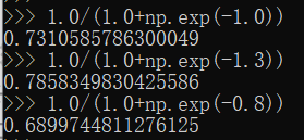
四舍五入后就得到了输入层的输出,输入层的输出就是隐藏层的输入。推广一下,其实就是上一层的输出是下一层的输入。

这句话也对应着论文里的描述:

The simplest form of the learning procedure is for layered networks which have a layer of input units at the bottom; any number of intermediate layers; and a layer of output units at the top. Connections within a layer or from higher to lower layers are forbidden, but connections can skip intermediate layers. An input vector is presented to the network by setting the states of the input units. Then the states of the unils in each layer are determined by applying equations (1) and (2) to the connections coming from lower layers. All units within a layer have their states set in parallel, but diferent layers have their states set sequentially, starting at the bottom and working upwards until the states of the output units are determined.

作者随后又说,其实没必要完全使用前面的公式(1)和公式(2):

It is not necessary to use exactly the functions given in equations (1) and (2). Any input-output function which has a bounded derivative will do. However, the use of a linear function for combining the inputs to a unit before applying the nonlinearity greatly simplifes the learning procedure.

并解释了这样做的目的:

The aim is to find a set of weights that ensure that for each input vector the output vector produced by the network is the same as (or suficiently close to) the desired output vector. If there is a fixed, finite set of input-output cases, the total error in the performance of the network with a particular set of weights can be computed by comparing the actual and desired output vectors for every case.

其实模型训练的过程就是找到一组合适的权重,使得网络的输出与预期的输出一致或者说足够接近预期输出

这里作者给出了第三个公式,用来计算total error, E:

• E = $\frac{1}{2}$ $\sum_{c}$ $\sum_{j}(y_{jc}-d_{jc})^2$     (3)

解释一下,d是指预期的输出值,y是网络的输出值

这一步其实不难理解,既然要反复调整网络的参数,那就要知道现在网络的效果和预期差多少,这个差值其实就是E,找到这个差值后,怎么去调整参数呢?

这里多提一句,到目前为止,描述的都是前向传播,正如作者在论文中描述的那样:

The forward pass in which the units in each layer have their states determined by the input they receive ftom units in lower layers using equations (1) and (2). The backward pass which propagates derivatives from the top layer back to the bottom one is more complicated.

反向传播具体怎么做呢?

作者给出的方法是先求方程E对y的偏导数:

The backward pass starts by computing ∂E/∂y for each of the output units.

可以得到第四个公式:

$∂E/∂y_j​ = y_j​ − d_j$​            (4)

根据链式法则可得到:

$∂E/∂x_j$​ = $∂E/∂y_j​$ $\cdot$ $dy_j/dx_j$

根据公式(2)又可以得到 $dy_j/dx_j$ = $y_j(1 - y_j)$

因此可以得到第五个公式:

$∂E/∂x_j$​ = $∂E/∂y_j​$ $\cdot$ $y_j(1 - y_j)$      (5)

通过上面这个公式,我们便可以知道某一层的输出x的变化将如何影响误差E

不难算出改变某一层的权重时,对误差的影响,这是第六个公式:

$∂E/∂w_{ji}$​ = $∂E/∂x_i$ $\cdot$ $∂x_j/∂w_{ji}$ = $∂E/∂x_j$ $\cdot$ $y_i$     (6)

某一层对上一层的影响简单来说就是:

$∂E/∂x_j$ $\cdot$ $∂x_j/∂y_i$ = $∂E/∂x_j$ $\cdot$ $w_{ji}$

把每一层的神经元相加,可以得到第七个公式:

$∂E/∂y_i$ = $\sum_{j}∂E/∂x_j$ $\cdot$ $w_{ji}$     (7)

我觉得难点到这里就算结束了,作者在这里说,得到最后一层的误差后,不难可以推出前几层的误差:

We have now seen how to compute $∂E/∂y_i$ for any unit in the penultimate layer when given $∂E/∂y_i$ for all units in the last layer. We can therefore repeat this procedure to compute this term for successively earlier layers, computing $∂E/∂w$ for the weights as we go.

计算出误差后,我们要去调整权重,这是比较重要的一步,作者提出了两种方法:

One way of using $∂E/∂w$ is to change the weights after every inpu-output case. This has the advantage that no separate memory is required for the derivatives. An alternative scheme, which we used in the research reported here, is to accumulate $∂E/∂w$ over all the input-output cases before changing the weights. The simplest version of gradient descent is to change. each weight by an amount proportional to the accumulated $∂E/∂w$

作者给出的是第二种方法,这是第8个公式:

Δw = -ε $∂E/∂w$     (8)

不过第二种方式的速度比较慢,作者提出了一种新方法:

It can be significantly improved, without sacrifcing the, simplicity and locality, by using an acceleration method in which the current gradient is used to modifty the velocity of the point in weight space instead of its position

这就是论文中的第九个公式,也是最后一个公式:

Δw(t) = − $ε∂E/∂w(t) + αΔw(t−1)$$     (9)

作者讲解了 t 和 α 的作用:

where t is incremented by 1 for each sweep through the whole set of input-output cases, and a is an exponential decay factor between 0 and 1 that determines the relative contribution of the current gradient and earlier gradients to the weight change.To break symmetry we start with small random weights.

到这里,整篇论文就接近尾声了,可能后面的那几个公式会让人头疼,这里我用excel表给大家做个简化,不用求偏导

还是用那个例子吧,输入一个数,输出它的相反数:

1. 假设权重weight初始为1
2. 输出等于输入乘权重即output = input * weight
3. 误差等于输出减去预期即error = output - expect
4. 防止权重变化的过快,于是设置学习率Learning rate为0.01
5. 下一轮的权重取决于上一轮的误差与学习率即weight = weight - error * Learning rate

补充一下表格(刚刚学习率设置得有点低,现在调整为0.1):

虽然error看上去是越来越大,但权重weight其实是在逐渐趋近于预期的(要输出相反数,权重应该为-1)

以上就是我对反向传播算法的理解,另外,我在阅读原文的过程中总结了一些高频词汇,希望能对大家在阅读原文时有所帮助:

• back-propagating 反向传播
• neurone-like units 类神经元
• task 任务
• attempt 尝试
• self-organizing neural network 自组神经网络
• vector 矢量
• input unit 输入层(只含有一个单元的层也算是一层)
• hidden unit 隐藏层
• output unit 输出层
• feature 特征
• at the bottom 在底部
• layer 层
• forbidden 禁止
• linear function 线性函数
• to minimize 使最小
• so as to 以便
• as a result of 由于
• the aim is to 目的是
• in order to 为了
• the difference between A and B A与B之间的区别

关于unit和layer的区别,我的理解是最小的layer是一个unit,所以我认为一个单元也可以算作一层,虽然这样有点不太恰当,不过可以当作包含关系吧