Graph Attention Networks网络结构+代码

论文
Tensorflow代码
pytorch代码

1. 创新点

通过新型神经网络对图形结构数据进行操作，利用隐藏的自注意层赋予邻域节点不同重要性，并无需提前了解整个网络结构

通过堆叠这样的一些层，这些层里的节点能够注意其邻近节点的特征，不需要进行成本高昂的矩阵运算（例如反演），也无需事先知道图的结构

1.1. attention 引入目的

• 为每个节点分配不同权重
• 关注那些作用比较大的节点，而忽视一些作用较小的节点
• 在处理局部信息的时候同时能够关注整体的信息，不是用来给参与计算的各个节点进行加权的，而是表示一个全局的信息并参与计算

1.2. 框架特点

• attention 计算机制高效，为每个节点和其每个邻近节点计算attention 可以并行进行
• 能够按照规则指定neighbor 不同的权重，不受邻居数目的影响
• 可直接应用到归纳推理问题中

2. 模型

2.1. feature 处理

通过线性变换生成新的更强的 feature
输入：node feature的集合

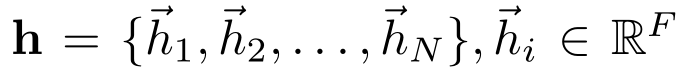
（ N 为node 数量, F 为每个node 的 feature 数–feature vector 长度）
输出：

（ 使用W 将每个特征转换为可用的表达性更强的特征）

2.2. 计算相互关注

每两个node 间都有了相互关注机制（用来做加权平均，卷积时，每个node 的更新是其他的加权平均
共享的关注机制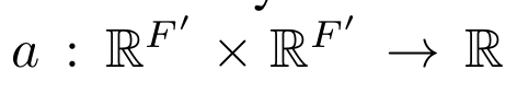
通过node feature 计算两个node 间的关系

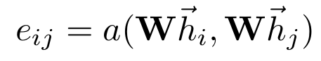
用来做加权平均需要转换一下参数

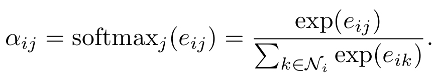
（这个系数 α 就是每次卷积时，用来进行加权求和的系数）

本文采取的计算attention coefficient的函数a是一个单层的前馈网络，LeakyReLU 处理得

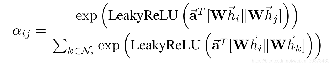
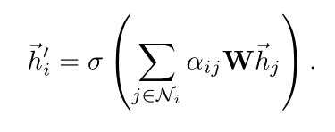
（ || 表示串联/ 连接，一旦获得，归一化的相互注意系数用来计算对应特征的线性组合，以用作每个节点的最终输出特征）

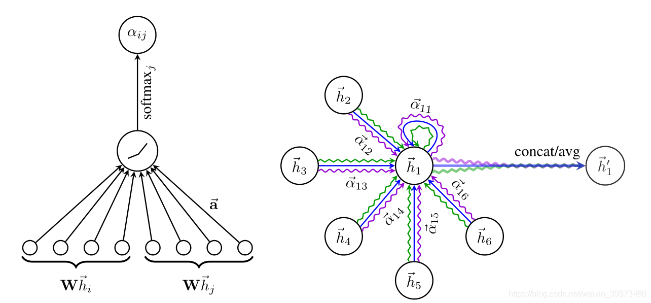
左图：
在模型中应用注意机制 $a(Wh_i||Wh_j)$，通过权重向量 a 参数化，应用 LeakyReLU 激活

右图：
节点 $h1'$在邻域中具有多端连接，不同的箭头样式表示独立的注意力计算，通过直连concat或平均avg获取 $h1'$。

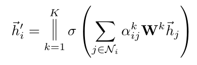
2.3 multi-head attention机制

• 不只用一个函数a进行attention coefficient的计算，而是设置K个函数，每一个函数都能计算出一组attention coefficient，并能计算出一组加权求和用的系数，每一个卷积层中，K个attention机制独立的工作，分别计算出自己的结果后连接在一起，得到卷积的结果，即
• 
• 假如有 k 个独立的相互注意机制同时计算，则集中其特征，可得到特征表示
  
• 对于最后一个卷积层，如果还是使用multi-head attention机制，那么就不采取连接的方式合并不同的attention机制的结果了，而是采用求平均的方式进行处理，即
  

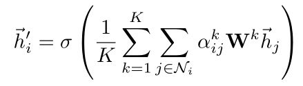
3.对比

• 计算很高效，attention机制在所有边上的计算是可以并行的，输出的feature的计算在所有节点上也可以并行
• 和GCN不同，本文的模型可以对同一个结点的相邻结点分配不同的重要性，使得模型的容量（自由度）大增。
• 分析这些学到的attentional weights有利于可解释性（可能是分析一下模型在分配不同的权重的时候是从哪些角度着手的）
• attention机制是对于所有edge共享的，不需要依赖graph全局的结构以及所有node的特征
• 2017年Hamilton提出的inductive method 对于neighborhood的模式处理固定，不灵活

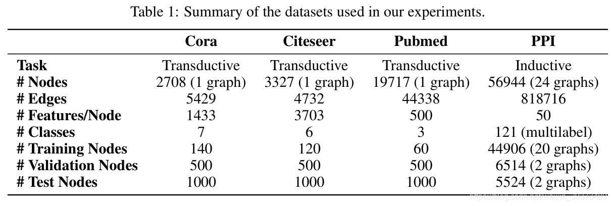
4.实验结果

5. 实现细节

5.1 代码解析

以pytorch版本的代码为例，解读如下：

• 读入数据：
  可见 Cora数据集介绍+读取
• 网络的总体架构

class GAT(nn.Module):
    def __init__(self, nfeat, nhid, nclass, dropout, alpha, nheads):
        """
        Dense version of GAT.
        :param nfeat: 输入特征的维度
        :param nhid:  输出特征的维度
        :param nclass: 分类个数
        :param dropout: dropout
        :param alpha: LeakyRelu中的参数
        :param nheads: 多头注意力机制的个数
        """
        super(GAT, self).__init__()
        self.dropout = dropout
        # 多头注意力机制
        self.attentions = [GraphAttentionLayer(nfeat, nhid, dropout=dropout, alpha=alpha, concat=True) for _ in range(nheads)]
        for i, attention in enumerate(self.attentions):
            self.add_module('attention_{}'.format(i), attention)
        # 输出层只用一个注意力机制
        self.out_att = GraphAttentionLayer(nhid * nheads, nclass, dropout=dropout, alpha=alpha, concat=False)

    def forward(self, x, adj):
        x = F.dropout(x, self.dropout, training=self.training) 
        x = torch.cat([att(x, adj) for att in self.attentions], dim=1) #(2708,64)
        x = F.dropout(x, self.dropout, training=self.training) 
        x = F.elu(self.out_att(x, adj)) 
        return F.log_softmax(x, dim=1)

• 注意力机制模块的实现

class GraphAttentionLayer(nn.Module): 
    """
    Simple GAT layer, similar to https://arxiv.org/abs/1710.10903
    """

    def __init__(self, in_features, out_features, dropout, alpha, concat=True):
        super(GraphAttentionLayer, self).__init__()
        self.dropout = dropout
        self.in_features = in_features
        self.out_features = out_features
        self.alpha = alpha
        self.concat = concat

        self.W = nn.Parameter(torch.zeros(size=(in_features, out_features)))
        nn.init.xavier_uniform_(self.W.data, gain=1.414)
        self.a = nn.Parameter(torch.zeros(size=(2*out_features, 1)))
        nn.init.xavier_uniform_(self.a.data, gain=1.414)

        self.leakyrelu = nn.LeakyReLU(self.alpha)

    def forward(self, input, adj):
        '''
        :param input: 输入特征 (batch,in_features)
        :param adj:  邻接矩阵 (batch,batch)
        :return: 输出特征 (batch,out_features)
        '''
        h = torch.mm(input, self.W) # (batch,out_features)
        N = h.size()[0] # batch
        # 将不同样本之间两两拼接，形成如下矩阵
        # [[结点1特征，结点1特征],
		#  [结点1特征，结点2特征],
		#   ......
		#  [结点1特征，结点j特征],
		#  [结点2特征，结点1特征],
		#  [结点2特征，结点2特征],
		#   ......
		#   ]
        a_input = torch.cat([h.repeat(1, N)   # (batch,out_features*batch)
                            .view(N * N, -1), # (batch*batch,out_features)
                             h.repeat(N, 1)], # (batch*batch,out_features)
                            dim=1).view(N, -1, 2 * self.out_features) # (batch,batch,2 * out_features)
        # 通过刚刚的矩阵与权重矩阵a相乘计算每两个样本之间的相关性权重，最后再根据邻接矩阵置零没有连接的权重
        e = self.leakyrelu(torch.matmul(a_input, self.a).squeeze(2)) # (batch,batch)
        # 置零的mask
        zero_vec = -9e15*torch.ones_like(e) # (batch,batch)
        attention = torch.where(adj > 0, e, zero_vec) # (batch,batch) 有相邻就为e位置的值，不相邻则为0
        attention = F.softmax(attention, dim=1)  # (batch,batch)
        attention = F.dropout(attention, self.dropout, training=self.training) # (batch,batch)
        h_prime = torch.matmul(attention, h) # (batch,out_features)

        if self.concat:
            return F.elu(h_prime)
        else:
            return h_prime

5.2 其他细节

transductive learning

• 两层 GAT
• 在Cora 数据集上优化网络结构的超参数，应用到Citeseer 数据集
• 第一层 8 head, F`=8 ELU 作为非线性函数
• 第二层为分类层，一个 attention head 特征数C，后跟 softmax 函数
• 为了应对小训练集，正则化（L2)
• 两层都采用 0.6 的dropout
• 相当于计算每个node位置的卷积时都是随机的选取了一部分近邻节点参与卷积

inductive learning

• 三层GAT 模型
• 前两层 K=4, F1=256 ELU作为非线性函数
• 最后一层用来分类 K=6, F`=121 后跟logistics sigmoid 激活函数
• 该任务中，训练集足够大不需要使用 正则化 和 dropout
• 两个任务都是用Glorot初始化初始的，并且是用Adam SGD来最小化交叉熵进行优化

参考
https://www.cnblogs.com/chaoran/p/9720708.html