吴恩达机器学习课后习题01-线性回归（01-linear regression）

吴恩达机器学习课后习题01-线性回归（01-linear regression）

切记！！！下载第一次课后作业的题目和数据包ex1data1.txt和ex1data2.txt，数据包一定要下载，并且导入到项目所在文件夹，用Ancona或者pycharm编译都可以成功！

（后续会慢慢补充并且完善线性回归知识点）

一、单变量线性回归

训练集，拟合（假设，陈述，代价函数），梯度下降法
损失函数，梯度下降函数，维度

案例：假设你是一家餐厅的CEO，正在考虑开一家分店，根据该人口数据测试其利润。

我们拥有不同城市对应的人口数据以及利润：ex1data1.txt

# 读取文件：
import numpy as np
import pandas as pd
import matplotlib.pyplot as plt

data = pd.read_csv('ex1data1.txt',names = ['population','profit'])
data.head()

data.tail()

data.describe()

data.info()

# 数据集准备：
data.plot.scatter('population','profit',label = 'population')
plt.show()

data.insert(0,'ones',1)
data.head()

X = data.iloc[:,0:-1]
X.head()

y = data.iloc[:,-1]
y.head()

X = X.values

X.shape

y = y.values

y.shape

# 损失函数：
y = y.reshape(97,1)
y.shape

def costFunction(X,y,theta):
    inner = np.power(X @ theta - y,2)
return np.sum(inner)/(2 * len(X))

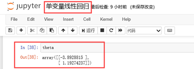
theta = np.zeros((2,1))
theta.shape

cost_init = costFunction(X,y,theta)
print(cost_init)

# 梯度下降函数：
def gradientDescent(X,y,theta,alpha,iters):
    costs = []
    
    for i in range(iters):
        theta = theta - (X.T @ (X@theta - y)) * alpha/len(X)
        cost = costFunction(X,y,theta)
        costs.append(cost)
        
        if i % 100 == 0:
            print(cost)
return theta,costs

alpha = 0.02
iters = 2000

theta,costs = gradientDescent(X,y,theta,alpha,iters)

# 可视化损失函数：
fig,ax = plt.subplots()
ax.plot(np.arange(iters),costs)
ax.set(xlabel = 'iters',
      ylabel = 'cost',
      title = 'cost vs iters')
plt.show()

fig,ax = plt.subplots(2,3)
ax1 = ax[0,0]
ax1.plot
plt.show()

# 拟合函数可视化：
x = np.linspace(y.min(),y.max(),100)
y_ = theta[0,0] + theta[1,0] * x

fig,ax = plt.subplots()
ax.scatter(X[:,-1],y,label = 'training data')
ax.plot(x,y_,'r',label = 'predict')
ax.legend()
ax.set(xlabel = 'populaition',
      ylabel = 'profit')
plt.show()

二、多变量线性回归

数据预处理（特征归一化、标准化、最大最小值），正规方程，梯度下降和正规方程比较

案例：假设你现在打算卖房子，想知道房子能卖多少钱？

我们拥有房子面积和卧室数量以及房子价格之间的对应函数数据：ex1data2.txt

# 读取文件：
import numpy as np
import pandas as pd
import matplotlib.pyplot as plt

data = pd.read_csv('ex1data2.txt',names = ['size','bedrooms','price'])
data.head()

# 特征归一化;
def normalize_feature(data):
return (data - data.mean()) / data.std()

data = normalize_feature(data)

data.head()

# 构造数据集：
data.plot.scatter('size','price',label = 'size')
plt.show()

data.plot.scatter('bedrooms','price',label = 'bedrooms')
plt.show()

# 添加全为1的列：
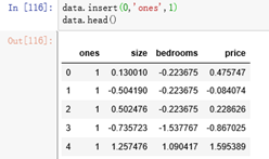
data.insert(0,'ones',1)
data.head()

# 构造数据集：
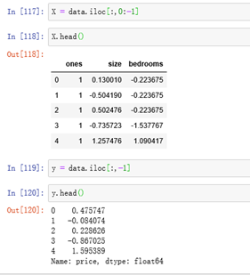
X = data.iloc[:,0:-1]

X.head()

y = data.iloc[:,-1]

y.head()

# 将dataframe转成数组：
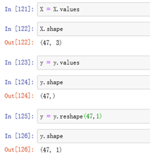
X = X.values

X.shape

y = y.values

y.shape

y = y.reshape(47,1)

y.shape

# 损失函数：
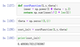
def costFunction(X,y,theta):
    inner = np.power(X @ theta - y,2)
return np.sum(inner)/(2 * len(X))

theta = np.zeros((3,1))

cost_init = costFunction(X,y,theta)

print(cost_init)

# 梯度下降函数：
def gradientDescent(X,y,theta,alpha,iters):
    costs = []
    
    for i in range(iters):
        theta = theta - (X.T @ (X@theta - y)) * alpha/len(X)
        cost = costFunction(X,y,theta)
        costs.append(cost)
        
        if i % 100 == 0:
            print(cost)
return theta,costs

# 不同alpha下的迭代效果：
candinate_alpha = [0.0003,0.003,0.03,0.0001,0.001,0.01]
iters = 2000

fig,ax = plt.subplots()

for alpha in candinate_alpha:
    _,costs = gradientDescent(X,y,theta,alpha,iters)
    ax.plot(np.arange(iters),costs,label = alpha)
    ax.legend()
     
ax.set(xlabel = 'iters',
      ylabel = 'cost',
      title = 'cost vs iters')
plt.show()

三、正规方程

import numpy as np
import pandas as pd
import matplotlib.pyplot as plt

data = pd.read_csv('ex1data1.txt',names = ['population','profit'])

data.insert(0,'ones',1)

X = data.iloc[:,0:-1]
y = data.iloc[:,-1]

X = X.values

y = y.values

y = y.reshape(97,1)

X.shape

y.shape

def normalEquation(X,y):
    theta = np.linalg.inv(X.T@X)@X.T@y
return theta

theta = normalEquation(X,y)

print(theta)

四、附录

完整代码：

单变量

# 读取文件
import numpy as np
import pandas as pd
import matplotlib.pyplot as plt

data = pd.read_csv('ex1data1.txt',names = ['population','profit'])
data.head()

data.tail()

data.describe()

data.info()

# 数据集准备
data.plot.scatter('population','profit',label = 'population')
plt.show()

data.insert(0,'ones',1)
data.head()

X = data.iloc[:,0:-1]
X.head()

y = data.iloc[:,-1]
y.head()

X = X.values

X.shape

y = y.values

y.shape

# 损失函数
y = y.reshape(97,1)
y.shape

def costFunction(X,y,theta):
    inner = np.power(X @ theta - y,2)
    return np.sum(inner)/(2 * len(X))

theta = np.zeros((2,1))
theta.shape

cost_init = costFunction(X,y,theta)
print(cost_init)

# 梯度下降函数：

def gradientDescent(X, y, theta, alpha, iters):
    costs = []

    for i in range(iters):
        theta = theta - (X.T @ (X @ theta - y)) * alpha / len(X)
        cost = costFunction(X, y, theta)
        costs.append(cost)

        if i % 100 == 0:
            print(cost)


    return theta, costs

alpha = 0.02
iters = 2000

theta, costs = gradientDescent(X, y, theta, alpha, iters)

# 可视化损失函数：
fig,ax = plt.subplots()
ax.plot(np.arange(iters),costs)
ax.set(xlabel = 'iters',
      ylabel = 'cost',
      title = 'cost vs iters')
plt.show()

fig,ax = plt.subplots(2,3)
ax1 = ax[0,0]
ax1.plot
plt.show()

# 拟合函数可视化：
x = np.linspace(y.min(),y.max(),100)
y_ = theta[0,0] + theta[1,0] * x

fig,ax = plt.subplots()
ax.scatter(X[:,-1],y,label = 'training data')
ax.plot(x,y_,'r',label = 'predict')
ax.legend()
ax.set(xlabel = 'populaition',
      ylabel = 'profit')
plt.show()

多变量

# 读取文件：
import numpy as np
import pandas as pd
import matplotlib.pyplot as plt

data = pd.read_csv('ex1data2.txt',names = ['size','bedrooms','price'])
data.head()

# 特征归一化;
def normalize_feature(data):
    return (data - data.mean()) / data.std()

data = normalize_feature(data)

data.head()

# 构造数据集：
data.plot.scatter('size','price',label = 'size')
plt.show()

data.plot.scatter('bedrooms','price',label = 'bedrooms')
plt.show()

# 添加全为1的列：
data.insert(0,'ones',1)
data.head()
# 构造数据集：
X = data.iloc[:,0:-1]

X.head()

y = data.iloc[:,-1]

y.head()
# 将dataframe转成数组：
X = X.values

X.shape

y = y.values

y.shape

y = y.reshape(47,1)

y.shape
# 损失函数：
def costFunction(X,y,theta):
    inner = np.power(X @ theta - y,2)
    return np.sum(inner)/(2 * len(X))

theta = np.zeros((3,1))

cost_init = costFunction(X,y,theta)

print(cost_init)

# 梯度下降函数：
def gradientDescent(X, y, theta, alpha, iters):
    costs = []

    for i in range(iters):
        theta = theta - (X.T @ (X @ theta - y)) * alpha / len(X)
        cost = costFunction(X, y, theta)
        costs.append(cost)

        if i % 100 == 0:
            print(cost)


    return theta, costs

# 不同alpha下的迭代效果：
candinate_alpha = [0.0003, 0.003, 0.03, 0.0001, 0.001, 0.01]
iters = 2000

fig, ax = plt.subplots()

for alpha in candinate_alpha:
    _, costs = gradientDescent(X, y, theta, alpha, iters)
    ax.plot(np.arange(iters), costs, label=alpha)
    ax.legend()

ax.set(xlabel='iters',
       ylabel='cost',
       title='cost vs iters')
plt.show()

正规方程

import numpy as np
import pandas as pd
import matplotlib.pyplot as plt

data = pd.read_csv('ex1data1.txt',names = ['population','profit'])

data.insert(0,'ones',1)

X = data.iloc[:,0:-1]
y = data.iloc[:,-1]

X = X.values

y = y.values

y = y.reshape(97,1)

X.shape

y.shape

def normalEquation(X,y):
    theta = np.linalg.inv(X.T@X)@X.T@y
    return theta

theta = normalEquation(X,y)

print(theta)