机器学习之逻辑回归详解--01

Logistic Regression

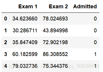
我们将建立一个逻辑回归模型来预测一个学生是否被大学录取。假设你是一个大学系的管理员，你想根据两次考试的结果来决定每个申请人的录取机会。你有以前的申请人的历史数据，你可以用它作为逻辑回归的训练集。对于每一个培训例子，你有两个考试的申请人的分数和录取决定。为了做到这一点，我们将建立一个分类模型，根据考试成绩估计入学概率。

import numpy as np
import pandas as pd
import matplotlib.pyplot as plt
import numpy.random
import time
import os

path =  'LogiReg_data.txt'
pdData = pd.read_csv(path, header=None, names=['Exam 1', 'Exam 2', 'Admitted'])
pdData.head() 

orig_data = pdData.as_matrix() 

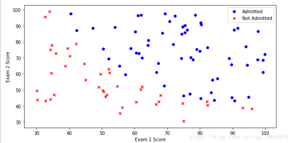
positive = pdData[pdData['Admitted'] == 1] # returns the subset of rows such Admitted = 1, i.e. the set of *positive* examples
negative = pdData[pdData['Admitted'] == 0] # returns the subset of rows such Admitted = 0, i.e. the set of *negative* examples

fig, ax = plt.subplots(figsize=(10,5))
ax.scatter(positive['Exam 1'], positive['Exam 2'], s=30, c='b', marker='o', label='Admitted')
ax.scatter(negative['Exam 1'], negative['Exam 2'], s=30, c='r', marker='x', label='Not Admitted')
ax.legend()
ax.set_xlabel('Exam 1 Score')
ax.set_ylabel('Exam 2 Score')

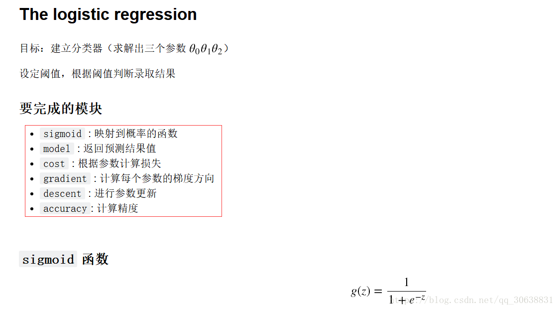
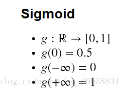
def sigmoid(z):
    return 1 / (1 + np.exp(-z))

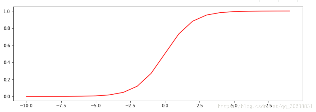
函数图像为:

nums = np.arange(-10, 10, step=1) #creates a vector containing 20 equally spaced values from -10 to 10
fig, ax = plt.subplots(figsize=(12,4))
ax.plot(nums, sigmoid(nums), 'r')

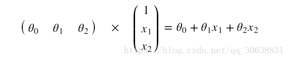
def model(X, theta):
    return sigmoid(np.dot(X, theta.T))

关于X,Y数据的处理:

orig_data = pdData.as_matrix() #原始数据

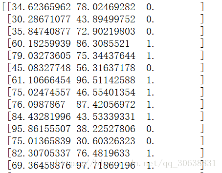
X矩阵的构造:

cols = orig_data.shape[1]

X = orig_data[:,0:cols-1]

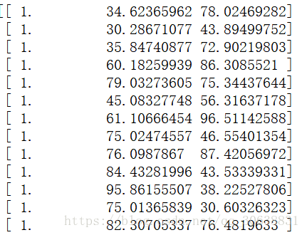
len1 = np.shape(X)[0]

X = np.c_[np.ones(len1),X]

y的构造：

y = orig_data[:,cols-1:cols]

theta的初始化:

theta = np.zeros([1, 3])

X.shape, y.shape, theta.shape

((100, 3), (100, 1), (1, 3))

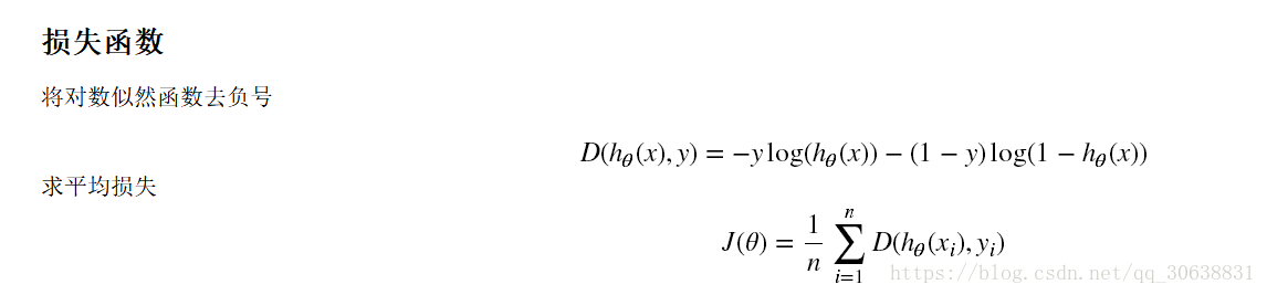
损失函数(造价函数)：

def cost(X, y, theta):
    left = np.multiply(-y, np.log(model(X, theta)))
    right = np.multiply(1 - y, np.log(1 - model(X, theta)))

    #print(type(np.sum(left - right)))
    return float(np.sum(left - right)) / (X.shape[0]) * 1.0

cost(X, y, theta)

返回结果:0.6931471805599453

def gradient(X, y, theta):
    grad = np.zeros(theta.shape)
    error = (model(X, theta) - y).ravel()
    for j in range(len(theta.ravel())):  # for each parmeter
        term = np.multiply(error, X[:, j])
        grad[0, j] = np.sum(term) / len(X)

    return grad

Gradient descent

比较3中不同梯度下降方法:

STOP_ITER = 0
STOP_COST = 1
STOP_GRAD = 2
theta = np.zeros([1, 3])

def stopCriterion(type, value, threshold):
    #设定三种不同的停止策略
    if type == STOP_ITER:     return value > threshold
    elif type == STOP_COST:   return abs(value[-1]-value[-2]) < threshold
    elif type == STOP_GRAD:   return np.linalg.norm(value) < threshold

数据进行洗牌:

#洗牌
def shuffleData(data):
    np.random.shuffle(data)
    cols = data.shape[1]
    X = data[:, 0:cols-1]
    y = data[:, cols-1:]
    return X, y

完整的函数:

n=100

def descent(data, theta, batchSize, stopType, thresh, alpha):
    # 梯度下降求解

    init_time = time.time()
    i = 0  # 迭代次数
    k = 0  # batch
    X, y = shuffleData(data)

    print(X)
    grad = np.zeros(theta.shape)  # 计算的梯度

    len1 = np.shape(X)[0]
    X = np.c_[np.ones(len1), X]

    costs = [cost(X, y, theta)]  # 损失值

    while True:
        grad = gradient(X[k:k + batchSize], y[k:k + batchSize], theta)
        k += batchSize  # 取batch数量个数据
        if k >= n:
            k = 0
            X, y = shuffleData(data)  # 重新洗牌
            len1 = np.shape(X)[0]
            X = np.c_[np.ones(len1), X]
        theta = theta - alpha * grad  # 参数更新
        costs.append(cost(X, y, theta))  # 计算新的损失
        i += 1

        if stopType == STOP_ITER:
            value = i
        elif stopType == STOP_COST:
            value = costs
        elif stopType == STOP_GRAD:
            value = grad
        if stopCriterion(stopType, value, thresh): break

    return theta, i - 1, costs, grad, time.time() - init_time

def runExpe(data, theta, batchSize, stopType, thresh, alpha):
    #import pdb; pdb.set_trace();

    theta, iter, costs, grad, dur = descent(data, theta, batchSize, stopType, thresh, alpha)
    name = "Original" if (data[:,1]>2).sum() > 1 else "Scaled"
    name += " data - learning rate: {} - ".format(alpha)

    if batchSize==n: strDescType = "Gradient"
    elif batchSize==1:  strDescType = "Stochastic"
    else: strDescType = "Mini-batch ({})".format(batchSize)

    name += strDescType + " descent - Stop: "

    if stopType == STOP_ITER: strStop = "{} iterations".format(thresh)
    elif stopType == STOP_COST: strStop = "costs change < {}".format(thresh)
    else: strStop = "gradient norm < {}".format(thresh)

    name += strStop
    print("***{}\nTheta: {} - Iter: {} - Last cost: {:03.2f} - Duration: {:03.2f}s".format(
        name, theta, iter, costs[-1], dur))
    fig, ax = plt.subplots(figsize=(12,4))
    ax.plot(np.arange(len(costs)), costs, 'r')
    ax.set_xlabel('Iterations')
    ax.set_ylabel('Cost')
    ax.set_title(name.upper() + ' - Error vs. Iteration')
    plt.show()
    return theta

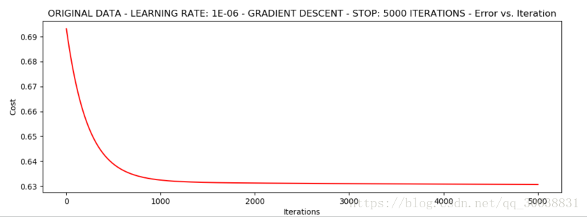
#选择的梯度下降方法是基于所有样本的

runExpe(orig_data, theta, n, STOP_ITER, thresh=5000, alpha=0.000001)

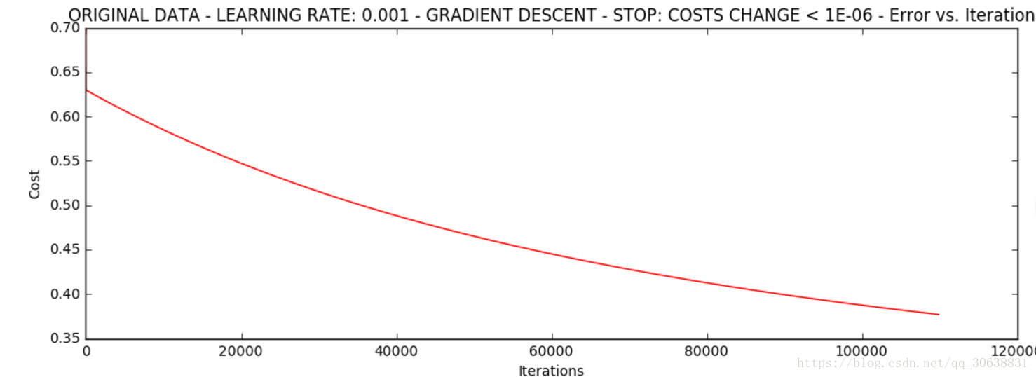
根据损失值停止

设定阈值 1E-6, 差不多需要110 000次迭代

runExpe(orig_data, theta, 1, STOP_COST, thresh=0.000001, alpha=0.001)

根据梯度变化停止

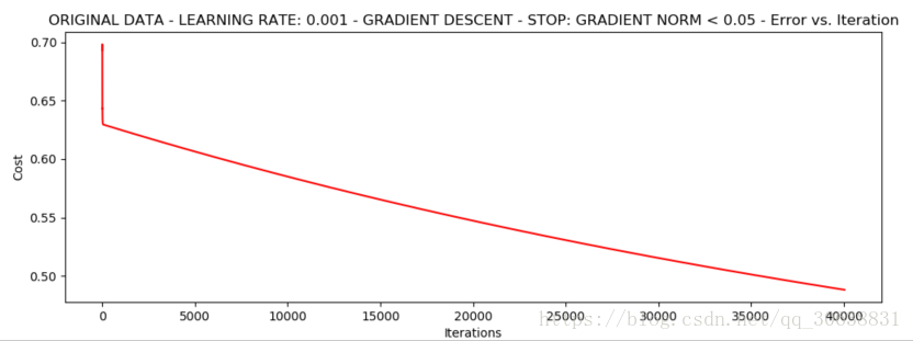
设定阈值 0.05,差不多需要40 000次迭代

runExpe(orig_data, theta, n, STOP_GRAD, thresh=0.05, alpha=0.001)

Stochastic descent

runExpe(orig_data, theta, 1, STOP_ITER, thresh=5000, alpha=0.001)

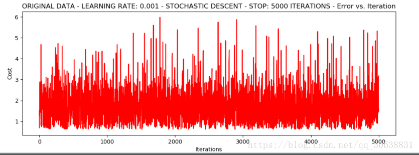
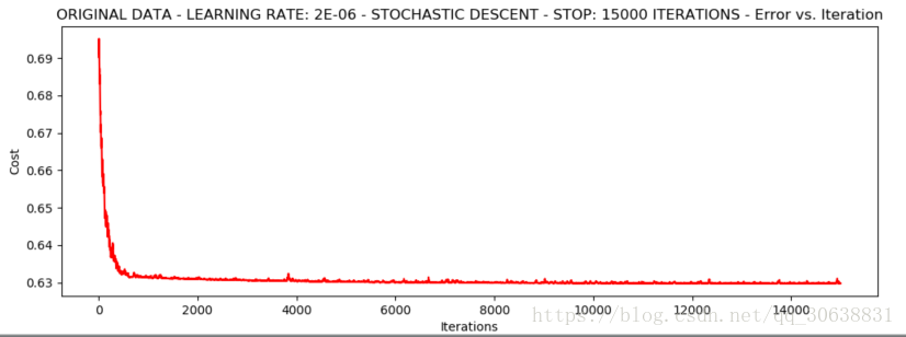
有点爆炸。。。很不稳定,再来试试把学习率调小一些

runExpe(orig_data, theta, 1, STOP_ITER, thresh=15000, alpha=0.000002)

Mini-batch descent

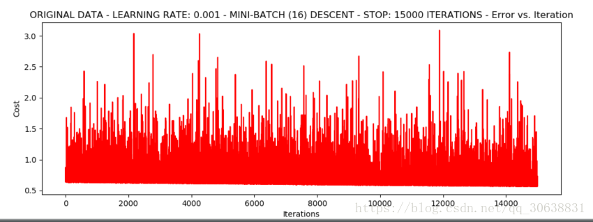
浮动仍然比较大，我们来尝试下对数据进行标准化 将数据按其属性(按列进行)减去其均值，然后除以其方差。最后得到的结果是，对每个属性/每列来说所有数据都聚集在0附近，方差值为1

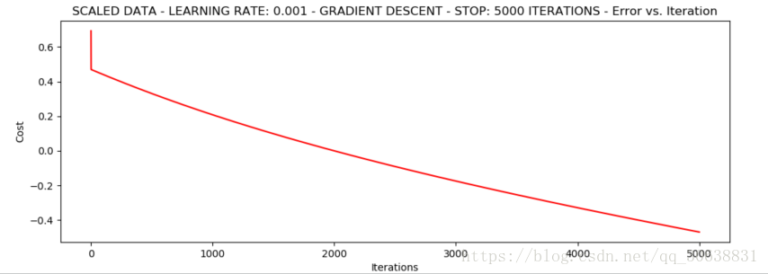
from sklearn import preprocessing as pp

scaled_data = orig_data.copy()
scaled_data[:, 1:3] = pp.scale(orig_data[:, 1:3])
print(orig_data)
print('-------------------------')
runExpe(scaled_data, theta, n, STOP_ITER, thresh=5000, alpha=0.001)

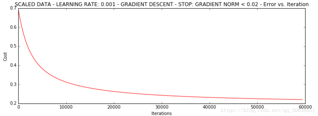
runExpe(scaled_data, theta, n, STOP_GRAD, thresh=0.02, alpha=0.001)

theta = runExpe(scaled_data, theta, 1, STOP_GRAD, thresh=0.002/5, alpha=0.001)

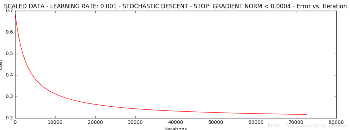
随机梯度下降更快，但是我们需要迭代的次数也需要更多，所以还是用batch的比较合适！！！

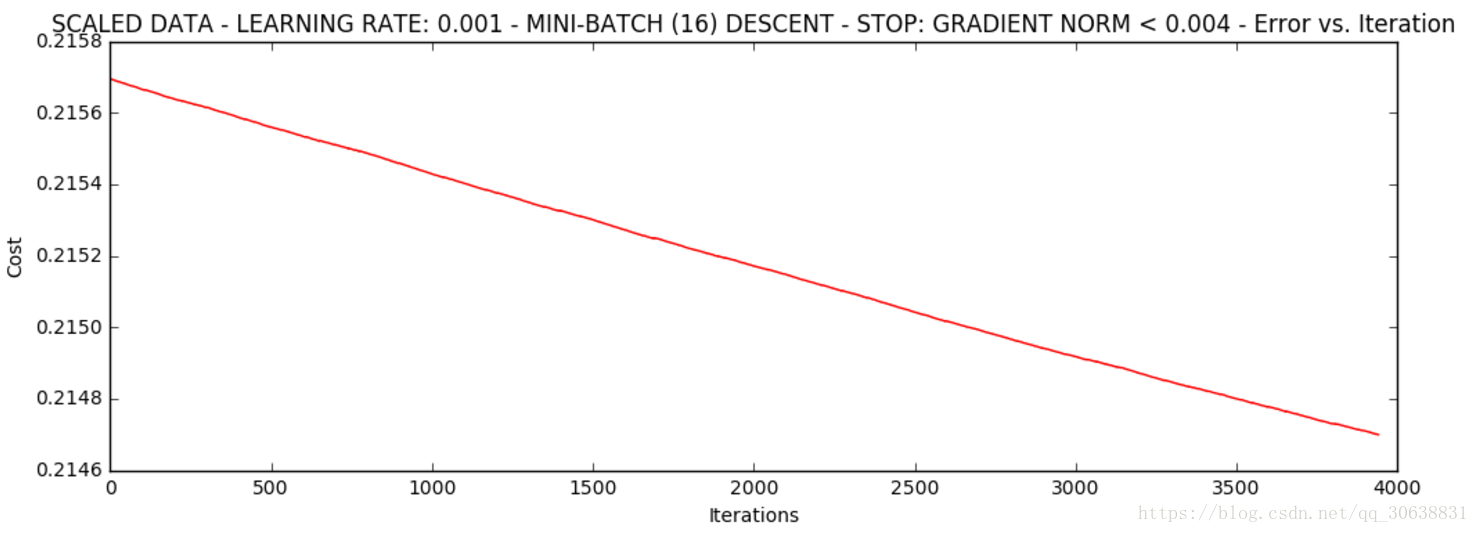
runExpe(scaled_data, theta, 16, STOP_GRAD, thresh=0.002*2, alpha=0.001)

精度:

#设定阈值
def predict(X, theta):
    return [1 if x >= 0.5 else 0 for x in model(X, theta)]


scaled_X = scaled_data[:, :3]
y = scaled_data[:, 3]
predictions = predict(scaled_X, theta)
correct = [1 if ((a == 1 and b == 1) or (a == 0 and b == 0)) else 0 for (a, b) in zip(predictions, y)]
accuracy = (sum(map(int, correct)) % len(correct))
print ('accuracy = {0}%'.format(accuracy))