浅层神经网络-图片识别-TF实现-数据可视化【人工智能学习】

我们在前文逻辑回归的基础上深入一下，使用浅层神经网络优化一下我们的学习方法

浅层神经网络：

浅层神经网络一般指的是只有一层隐藏层的神经网络
而神经网络的作用是通过多个学习单元的作用，来提高判断的准确率

换句话说，我们之前的回归判断相当于众多神经元当中的一个，我们需要通过多个这样的回归方程组建一个学习网络，这样他可以从更多的角度来去推测结果，这样的结果也会更加准确

而浅层神经网络一般是这样的：

上图就是我们今天要是实现的神经网络的图解了，这里面的【i[n ]】是指输入层，换句话说我们一口气输入的训练集数量。

如果按照非神经元件的做法，下一步就直接到out节点的输出层了，而我们在这里则多了一层h层（hide），这一层就是我们搭建的神经网络，本文中我们将构建1000个节点作为隐藏层。

通过多个节点学习公式的组合，体高精度，最后选取最后可能的结果使用softmax进行输出

值得注意的是，这里面涉及到了激活函数的概念，其实在之前的回归当中我们已经逐步涉及到了激活的相关概念，她的作用是：将原来的数据集当中的因变量、自变量的变化和相关性放大，详情请看ReLu函数的相关解析。

和昨天的逻辑回归一样，我们这里的每一层神经元最后还是要通过loss计算损失（交叉熵），再优化和迭代，最后使用Softmax函数进行输出。

代码实现

首先我们翻开之前的逻辑回归的相关代码：

#-*- coding:utf-8 -*-
import time
import numpy as np
import matplotlib.pyplot as plt
import tensorflow as tf
from tensorflow.examples.tutorials.mnist import input_data

MNIST = input_data.read_data_sets("./", one_hot=True)
cost_accum = []

learning_rate = 0.01
batch_size = 128
n_epochs = 25

X = tf.placeholder(tf.float32, [batch_size, 784])
Y = tf.placeholder(tf.float32, [batch_size, 10])

w = tf.Variable(tf.random_normal(shape=[784,10], stddev=0.01), name="weights")
b = tf.Variable(tf.zeros([1, 10]), name="bias")

logits = tf.matmul(X, w) + b

entropy = tf.nn.softmax_cross_entropy_with_logits(labels=Y, logits=logits)
loss = tf.reduce_mean(entropy)
optimizer = tf.train.GradientDescentOptimizer(learning_rate=learning_rate).minimize(loss)

init = tf.global_variables_initializer()

with tf.Session() as sess:
    sess.run(init)

    n_batches = int(MNIST.train.num_examples/batch_size)
    for i in range(n_epochs):
        for j in range(n_batches):
            X_batch, Y_batch = MNIST.train.next_batch(batch_size)
            loss_ = sess.run([optimizer, loss], feed_dict={ X: X_batch, Y: Y_batch})
            print("Loss of epochs[{0}] batch[{1}]: {2}".format(i, j, loss_))
            cost_accum.append(loss_)


    n_batches = int(MNIST.test.num_examples/batch_size)
    total_correct_preds = 0
    for i in range(n_batches):
        X_batch, Y_batch = MNIST.test.next_batch(batch_size)
        preds = tf.nn.softmax(tf.matmul(X_batch, w) + b) #算预测结果
        correct_preds = tf.equal(tf.argmax(preds, 1), tf.argmax(Y_batch, 1)) #判断预测结果和标准结果
        accuracy = tf.reduce_sum(tf.cast(correct_preds, tf.float32))#先转化判断的字符类型，再降维求和，这样就得到了一大堆压缩后的判断结果
        total_correct_preds += sess.run(accuracy) #之前都是公式，必须要run才有用，然后记录数量

    print("Accuracy {0}".format(total_correct_preds/MNIST.test.num_examples))#判断正确率并输出

plt.plot(range(len(cost_accum)), cost_accum, 'r')
plt.title('Logic Regression Cost Curve')
plt.xlabel('epoch*batch')
plt.ylabel('loss')
print('show')
plt.show()

我们对比前文的图可知，我们现在缺少的是将一个学习模型，变成多个并且组成隐藏层的函数。

参考上文代码中对于w、b的定义来规划一个快速制作单个节点的方法

w = tf.Variable(tf.random_normal(shape=[784,10], stddev=0.01), name="weights")
b = tf.Variable(tf.zeros([1, 10]), name="bias")

在这里我们需要怎家每个节点的输出值，我们定义为Z，Z的定义取代了前文我们logit的函数（就是那个logits = tf.matmul(X, w) + b），然后为在增加一个变量：激活函数（方便后续使用）
则得到下面的方法：

def add_layer(inputs ,in_size,out_size,activation_function= True):
    #初始化变量
    W = tf.Variable(tf.random_normal([in_size,out_size]))#初始化正态分布,in列，out行，第一层in传入784，第二层传入1000
    b = tf.Variable(tf.zeros([1,out_size])) #偏置量初始化，1列。out行

    Z = tf.matmul(inputs,W)+b #初始化公式，每一层都要有

     #为了防止报错，如果没有传入激活共识，则不作处理
    if activation_function is None:
        outputs = Z
    else:
        outputs = activation_function(Z)

    return outputs

并且在原来代码的基础上，将W、b的定义变成添加隐藏层和构建输出层，输入层不用构建，是因为直接由训练集输入的时候已经规定好的。

#初始化
X = tf.placeholder(tf.float32, [batch_size, 784])
Y = tf.placeholder(tf.float32, [batch_size, 10])
# 添加隐藏层
l1 = add_layer(X, 784, 1000, activation_function=tf.nn.relu)
pre = add_layer(l1, 1000, 10, activation_function=None)  # 输出
# w = tf.Variable(tf.random_normal(shape=[784,10], stddev=0.01), name="weights")
# b = tf.Variable(tf.zeros([1, 10]), name="bias")

# logits = tf.matmul(X, w) + b

OK，改造完成，把代码改好、调试完毕后（我增加了一点点显示效果罢了，无关痛痒）代码参考如下：

#-*- coding:utf-8 -*-
import numpy as np
import matplotlib.pyplot as plt
import tensorflow as tf
from tensorflow.examples.tutorials.mnist import input_data

def add_layer(inputs ,in_size,out_size,activation_function= True):
    #初始化变量
    W = tf.Variable(tf.random_normal([in_size,out_size]))#初始化正态分布,in列，out行，第一层in传入784，第二层传入1000
    b = tf.Variable(tf.zeros([1,out_size])) #偏置量初始化，1列。out行

    Z = tf.matmul(inputs,W)+b #初始化公式，每一层都要有

     #为了防止报错，如果没有传入激活共识，则不作处理
    if activation_function is None:
        outputs = Z
    else:
        outputs = activation_function(Z)

    return outputs

MNIST = input_data.read_data_sets("./", one_hot=True)
cost_accum = []

learning_rate = 0.05
batch_size = 128
n_epochs = 1

X = tf.placeholder(tf.float32, [batch_size, 784])
Y = tf.placeholder(tf.float32, [batch_size, 10])
# 添加隐藏层
l1 = add_layer(X, 784, 1000, activation_function=tf.nn.relu)
pre = add_layer(l1, 1000, 10, activation_function=None)  # 输出
# w = tf.Variable(tf.random_normal(shape=[784,10], stddev=0.01), name="weights")
# b = tf.Variable(tf.zeros([1, 10]), name="bias")

# logits = tf.matmul(X, w) + b

entropy = tf.nn.softmax_cross_entropy_with_logits(labels=Y, logits=pre)
loss = tf.reduce_mean(entropy)
optimizer = tf.train.AdamOptimizer(learning_rate=learning_rate).minimize(loss)
# optimizer = tf.train.GradientDescentOptimizer(learning_rate=learning_rate).minimize(loss)

init = tf.global_variables_initializer()

with tf.Session() as sess:
    sess.run(init)

    n_batches = int(MNIST.train.num_examples/batch_size)
    for i in range(n_epochs):
        for j in range(n_batches):
            X_batch, Y_batch = MNIST.train.next_batch(batch_size)
            loss_ = sess.run([optimizer, loss], feed_dict={ X: X_batch, Y: Y_batch})
            if j==0 :
                print("Loss oss of epochs[%s] batch[%s]: %s"%(i, j, loss_))
            cost_accum.append(loss_)


    n_batches = int(MNIST.test.num_examples/batch_size)
    total_correct_preds = 0
    for i in range(n_batches):
        X_batch, Y_batch = MNIST.test.next_batch(batch_size)
        # preds = tf.nn.softmax(tf.matmul(X_batch, w) + b)  # 算预测结果
        preds = sess.run(pre, feed_dict={X: X_batch, Y: Y_batch}) #算预测结果
        correct_preds = tf.equal(tf.argmax(preds, 1), tf.argmax(Y_batch, 1)) #判断预测结果和标准结果
        accuracy = tf.reduce_sum(tf.cast(correct_preds, tf.float32))#先转化判断的字符类型，再降维求和，这样就得到了一大堆压缩后的判断结果
        total_correct_preds += sess.run(accuracy) #之前都是公式，必须要run才有用，然后记录数量


    print("Accuracy {0}".format(total_correct_preds/MNIST.test.num_examples))#判断正确率并输出

plt.plot(range(len(cost_accum)), cost_accum, 'r')
plt.title('Logic Regression Cost Curve')
plt.xlabel('epoch*batch')
plt.ylabel('loss')
print('show')
plt.show()

代码运行结果如下（仅仅学习一个回合哦）：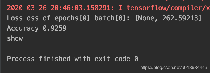

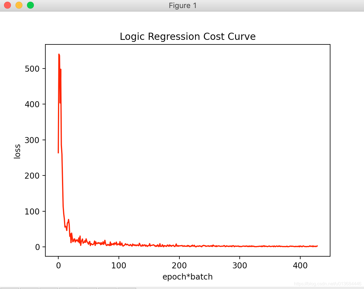
可以明显观察到位拟合速度快速提高，且学习后loss波动大幅减少，拟合率提高1个百分点。
那我们提高学习次数的结果呢：

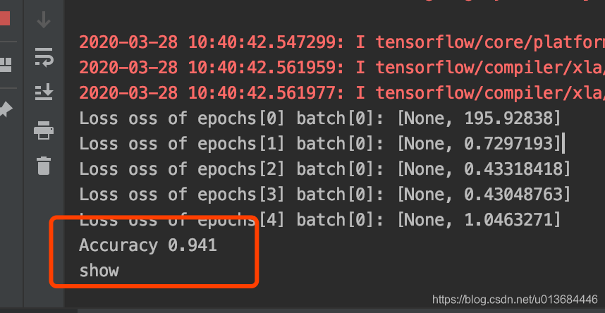
可以看到我们的学习结果有非常大的进步！
那我们把神经元的数量扩大呢，直接变成2000个隐藏层？

可以看到我们的进步很小，但是学习时间却非常的长，这样很不划算

那么除了增加学习次数意外，还有什么方法可以继续优化吗？
那么让我们快去期待一下深层神经网络吧。