本文将用孪生神经网络模型,对手写数字集minist进行相似度比较,用的框架是keras。如果还不清楚神经网络,可以看一下这篇文章神经网络 (caodong0225.github.io)。
MNIST是一个手写体数字的图片数据集,该数据集来由美国国家标准与技术研究所发起整理,一共统计了来自250个不同的人手写数字图片,其中50%是高中生,50%来自人口普查局的工作人员。该数据集的收集目的是希望通过算法,实现对手写数字的识别。
训练集一共包含了 60,000 张图像和标签,而测试集一共包含了 10,000 张图像和标签。测试集中前5000个来自最初NIST项目的训练集.,后5000个来自最初NIST项目的测试集。前5000个比后5000个要规整,这是因为前5000个数据来自于美国人口普查局的员工,而后5000个来自于大学生。
下载地址:caodong0225.github.io/minist.zip at master · caodong0225/caodong0225.github.io
该数据集自1998年起,被广泛地应用于机器学习和深度学习领域,用来测试算法的效果,例如线性分类器(Linear Classifiers)、K-近邻算法(K-Nearest Neighbors)、支持向量机(SVMs)、神经网络(Neural Nets)、卷积神经网络(Convolutional nets)等等。
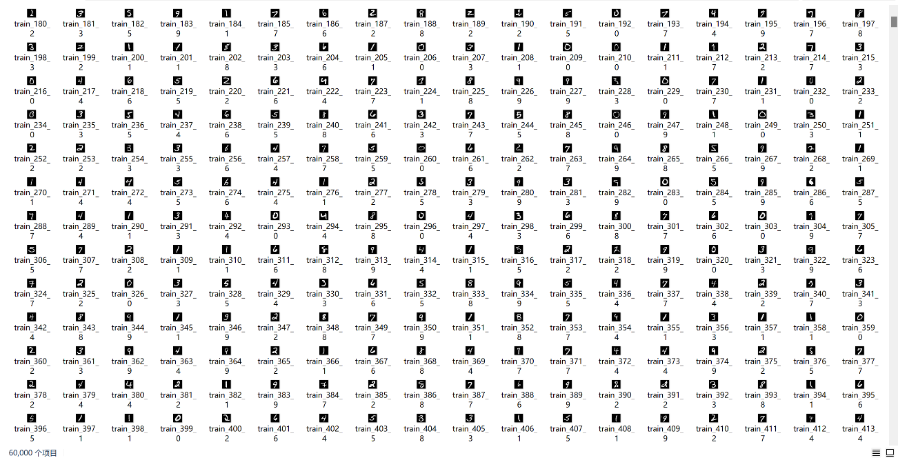
图1(minist部分手写数据集)
而Keras是一个由Python编写的开源人工神经网络库,可以作为Tensorflow、Microsoft-CNTK和Theano的高阶应用程序接口,进行深度学习模型的设计、调试、评估、应用和可视化 。
Keras在代码结构上由面向对象方法编写,完全模块化并具有可扩展性,其运行机制和说明文档有将用户体验和使用难度纳入考虑,并试图简化复杂算法的实现难度。Keras支持现代人工智能领域的主流算法,包括前馈结构和递归结构的神经网络,也可以通过封装参与构建统计学习模型。在硬件和开发环境方面,Keras支持多操作系统下的多GPU并行计算,可以根据后台设置转化为Tensorflow、Microsoft-CNTK等系统下的组件。因而本文用keras做为框架。
至于孪生神经网络(Siamese neural network),又名双生神经网络,是基于两个人工神经网络建立的耦合构架。孪生神经网络以两个样本为输入,输出其嵌入高维度空间的表征,以比较两个样本的相似程度。狭义的孪生神经网络由两个结构相同,且权重共享的神经网络拼接而成。广义的孪生神经网络,或“伪孪生神经网络(pseudo-siamese network)”,可由任意两个神经网拼接而成。孪生神经网络通常具有深度结构,可由卷积神经网络、循环神经网络等组成。
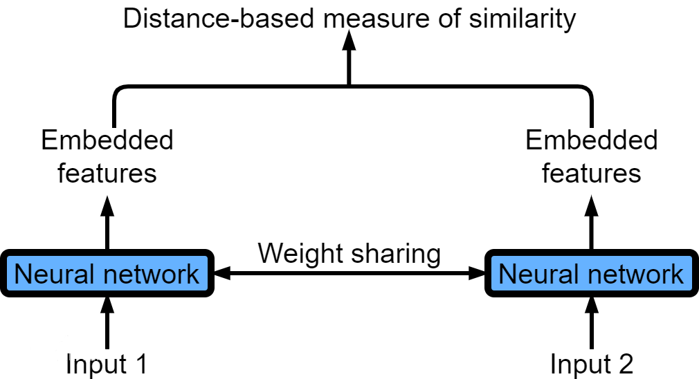
图2孪生神经网络示意图
所谓权值共享就是当神经网络有两个输入的时候,这两个输入使用的神经网络的权值是共享的(可以理解为使用了同一个神经网络)。很多时候,我们需要去评判两张图片的相似性,比如比较两张人脸的相似性,我们可以很自然的想到去提取这个图片的特征再进行比较,自然而然的,我们又可以想到利用神经网络进行特征提取。如果使用两个神经网络分别对图片进行特征提取,提取到的特征很有可能不在一个域中,此时我们可以考虑使用一个神经网络进行特征提取再进行比较。这个时候我们就可以理解孪生神经网络为什么要进行权值共享了。
孪生神经网络有两个输入(Input1 and Input2),利用神经网络将输入映射到新的空间,形成输入在新的空间中的表示。通过Loss的计算,评价两个输入的相似度。
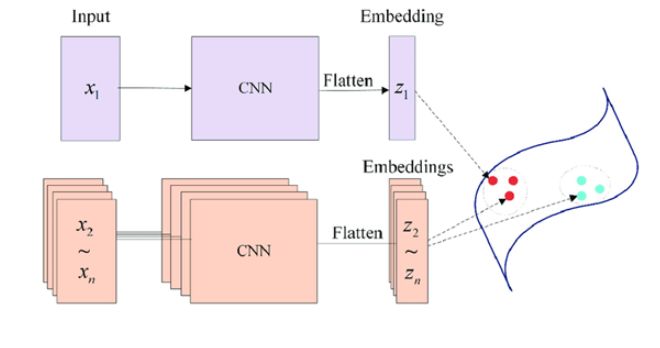
图3孪生神经网络示意图
映射的方法有多种,常见的映射方法为平方差映射和绝对值映射。对于输入的两张图片,在通过共享权重的神经网络的特征提取后,会得到两组一维,大小为N的特征向量W1,W2。设通过映射后得到的一维向量为W3,那么平方差映射的公式为:
![]()
绝对值映射的公式为:
![]()
至此,孪生神经网络共享权重的部分就结束了,对于新的向量W3,既可以继续进行神经网络操作,也可以将向量的每个值加起来后开平方或者取平均值做为损失函数,视具体情况而定。在本例中,我们采取后者方法,我们规定这个损失函数叫做对比损失函数(contrasive loss)。公式为:
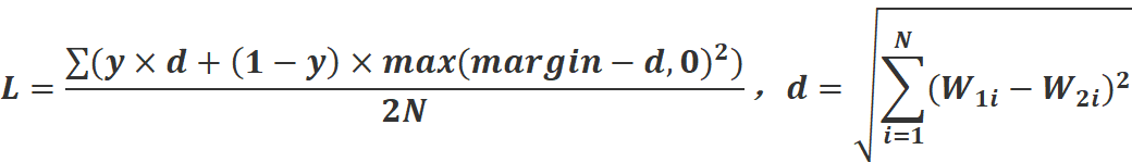
其中y表示样本标签,也就是1或者0,表示输入的两张图片是否为同一种类型的图片,如果是就为1,否则为0。margin表示阈值,因为当输入图片为不同类型时,d的值会非常大,为了防止d过大导致损失函数变化不均匀,所以设置阈值,一般margin的值取1。
观察这个式子可以发现,当输入图片为相同类型时,损失函数就是MSE损失函数开平方,神经网络会把W1,W2的值调整得尽量相等,从而d的值越小,损失函数的值越小。当输入图片为不同类型时,神经网络会把W1,W2的值调整得尽量不相等,从而d的值越大,如果d的值超过了阈值margin,那么损失函数的值就为0。
为了衡量模型在训练集上的准确度,对于Accuracy的计算也需要设计一个函数,在本例中,我们规定,当d>0.5时,神经网络将认定两张图片为不同图片,d<0.5时,神经网络将认定两张图片为同一图片。可视具体情况调整划分的值。
准确度的代码如下:
import keras.backend as K

def accuracy(y_true, y_pred): # Tensor上的操作

    return K.mean(K.equal(y_true, K.cast(y_pred < 0.5, y_true.dtype)))
损失函数的代码如下:
import keras.backend as K

def contrastive_loss(y_true, y_pred):

     margin = 1

     sqaure_pred = K.square(y_pred)

     margin_square = K.square(K.maximum(margin - y_pred, 0))

     return K.mean(y_true * sqaure_pred + (1 - y_true) * margin_square)
神经网络的结构构造如下:
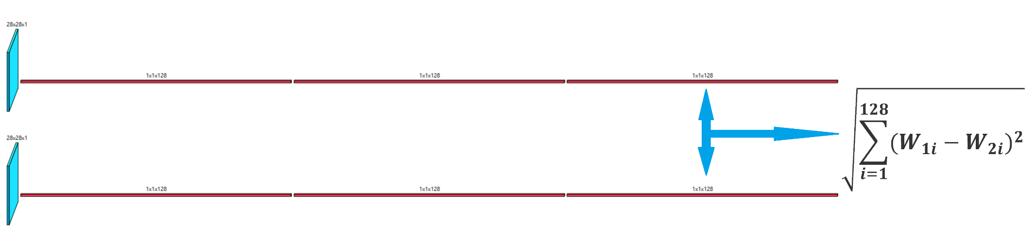
图4孪生神经网络构造图
完整的代码如下:
#coding:gbk

from keras.layers import Input,Dense

from keras.layers import Flatten,Lambda,Dropout

from keras.models import Model

import keras.backend as K

from keras.models import load_model

import numpy as np

from PIL import Image

import glob

import matplotlib.pyplot as plt

from PIL import Image

import random

from keras.optimizers import Adam,RMSprop

import tensorflow as tf

def create_base_network(input_shape):

    image_input = Input(shape=input_shape)

    x = Flatten()(image_input)

    x = Dense(128, activation='relu')(x)

    x = Dropout(0.1)(x)

    x = Dense(128, activation='relu')(x)

    x = Dropout(0.1)(x)

    x = Dense(128, activation='relu')(x)

    model = Model(image_input,x,name = 'base_network')

    return model

def contrastive_loss(y_true, y_pred):

     margin = 1

     sqaure_pred = K.square(y_pred)

     margin_square = K.square(K.maximum(margin - y_pred, 0))

     return K.mean(y_true * sqaure_pred + (1 - y_true) * margin_square)

def accuracy(y_true, y_pred): # Tensor上的操作

    return K.mean(K.equal(y_true, K.cast(y_pred < 0.5, y_true.dtype)))

def siamese(input_shape):

    base_network = create_base_network(input_shape)

    input_image_1 = Input(shape=input_shape)

    input_image_2 = Input(shape=input_shape)


    encoded_image_1 = base_network(input_image_1)

    encoded_image_2 = base_network(input_image_2)


    l2_distance_layer = Lambda(

        lambda tensors: K.sqrt(K.sum(K.square(tensors[0] - tensors[1]), axis=1, keepdims=True))

        ,output_shape=lambda shapes:(shapes[0][0],1))

    l2_distance = l2_distance_layer([encoded_image_1, encoded_image_2])


    model = Model([input_image_1,input_image_2],l2_distance)


    return model

def process(i):

    img = Image.open(i,"r")

    img = img.convert("L")

    img = img.resize((wid,hei))

    img = np.array(img).reshape((wid,hei,1))/255

    return img

#model = load_model("testnumber.h5",custom_objects={'contrastive_loss':contrastive_loss,'accuracy':accuracy})

wid=28

hei=28

model = siamese((wid,hei,1))

imgset=[[],[],[],[],[],[],[],[],[],[]]

for i in glob.glob(r"train_images\*.jpg"):

    imgset[int(i[-5])].append(process(i))

size = 60000


r1set = []

r2set = []

flag = []

for j in range(size):

    if j%2==0:

        index = random.randint(0,9)

        r1 = imgset[index][random.randint(0,len(imgset[index])-1)]

        r2 = imgset[index][random.randint(0,len(imgset[index])-1)]

        r1set.append(r1)

        r2set.append(r2)

        flag.append(1.0)

    else:

        index1 = random.randint(0,9)

        index2 = random.randint(0,9)

        while index1==index2:

            index1 = random.randint(0,9)

            index2 = random.randint(0,9)

        r1 = imgset[index1][random.randint(0,len(imgset[index1])-1)]

        r2 = imgset[index2][random.randint(0,len(imgset[index2])-1)]

        r1set.append(r1)

        r2set.append(r2)

        flag.append(0.0)

r1set = np.array(r1set)

r2set = np.array(r2set)

flag = np.array(flag)

model.compile(loss = contrastive_loss,

            optimizer = RMSprop(),

            metrics = [accuracy])

history = model.fit([r1set,r2set],flag,batch_size=128,epochs=20,verbose=2)

# 绘制训练 & 验证的损失值

plt.figure()

plt.subplot(2,2,1)

plt.plot(history.history['accuracy'])

plt.title('Model accuracy')

plt.ylabel('Accuracy')

plt.xlabel('Epoch')

plt.legend(['Train'], loc='upper left')

plt.subplot(2,2,2)

plt.plot(history.history['loss'])

plt.title('Model loss')

plt.ylabel('Loss')

plt.xlabel('Epoch')

plt.legend(['Train'], loc='upper left')

plt.show()

model.save("testnumber.h5")
训练过程图如下:
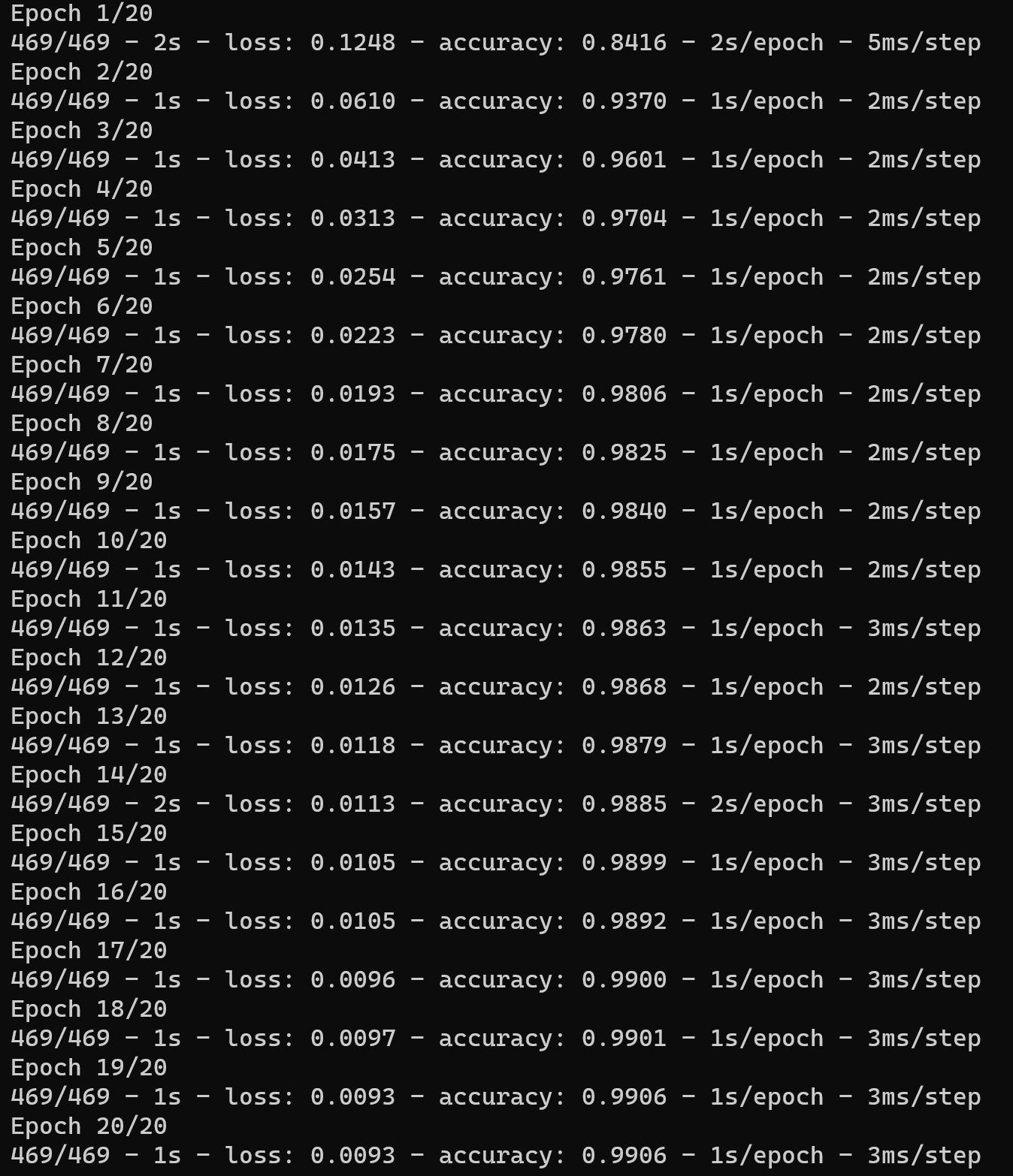
图5训练过程图
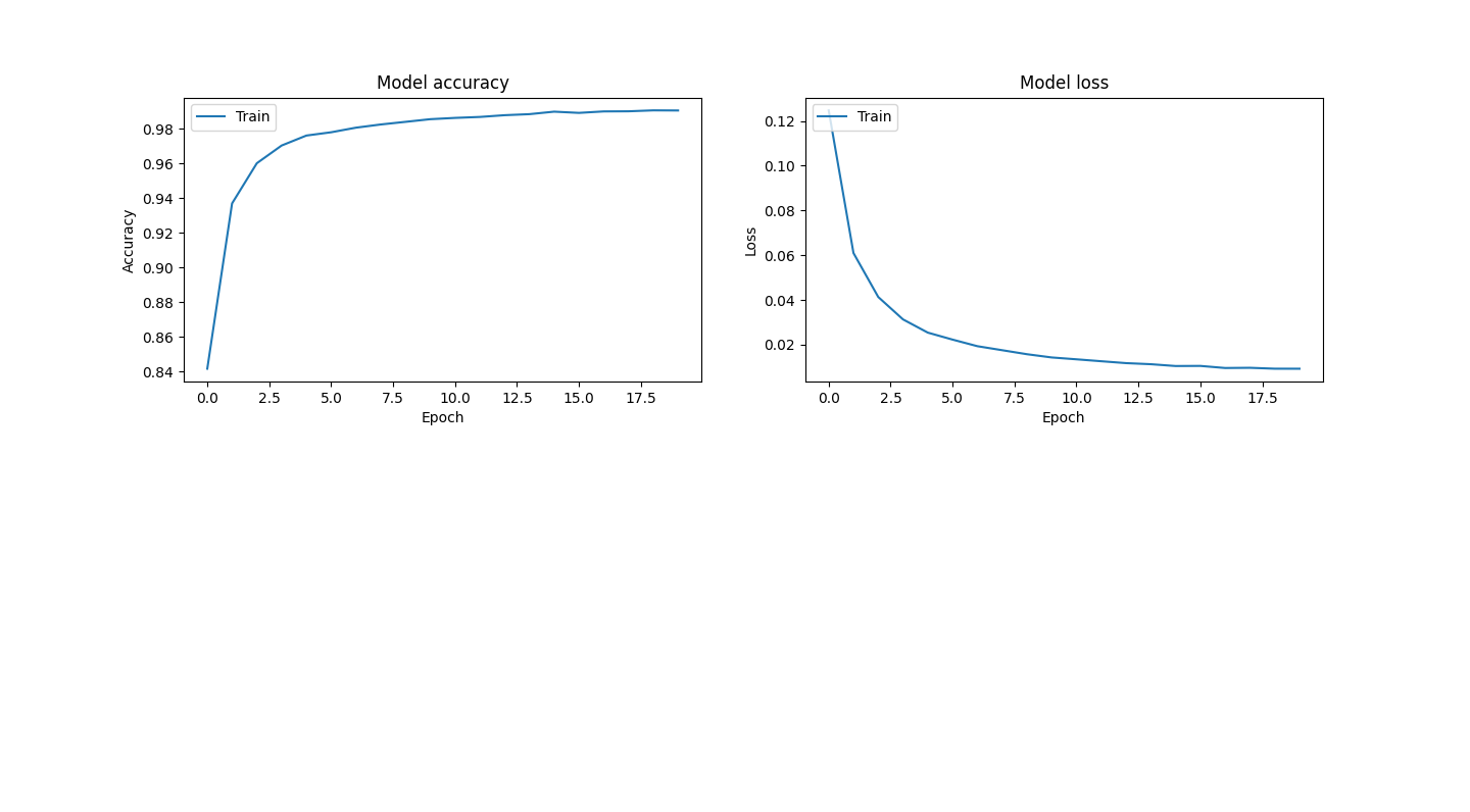
图6训练过程图
评估的展示代码如下:
import glob

from PIL import Image

import random

def process(i):

    img = Image.open(i,"r")

    img = img.convert("L")

    img = img.resize((wid,hei))

    img = np.array(img).reshape((wid,hei,1))/255

    return img

def contrastive_loss(y_true, y_pred):

     margin = 1

     sqaure_pred = K.square(y_pred)

     margin_square = K.square(K.maximum(margin - y_pred, 0))

     return K.mean(y_true * sqaure_pred + (1 - y_true) * margin_square)

def accuracy(y_true, y_pred): # Tensor上的操作

    return K.mean(K.equal(y_true, K.cast(y_pred < 0.5, y_true.dtype)))

def compute_accuracy(y_true, y_pred):

    pred = y_pred.ravel() < 0.5

    return np.mean(pred == y_true)

imgset=[]

wid = 28

hei = 28

imgset=[[],[],[],[],[],[],[],[],[],[]]

for i in glob.glob(r"test_images\*.jpg"):

    imgset[int(i[-5])].append(process(i))

model = load_model("testnumber.h5",custom_objects={'contrastive_loss':contrastive_loss,'accuracy':accuracy})

for i in range(50):

    if random.randint(0,1)==0:

        index=random.randint(0,9)

        r1 = random.randint(0,len(imgset[index])-1)

        r2 = random.randint(0,len(imgset[index])-1)

        plt.figure()

        plt.subplot(2,2,1)

        plt.imshow((255*imgset[index][r1]).astype('uint8'))

        plt.subplot(2,2,2)

        plt.imshow((255*imgset[index][r2]).astype('uint8'))

        y_pred = model.predict([np.array([imgset[index][r1]]),np.array([imgset[index][r2]])])

        print(y_pred)

        plt.show()

    else:

        index1 = random.randint(0,9)

        index2 = random.randint(0,9)

        while index1==index2:

            index1 = random.randint(0,9)

            index2 = random.randint(0,9)

        r1 = random.randint(0,len(imgset[index1])-1)

        r2 = random.randint(0,len(imgset[index2])-1)

        plt.figure()

        plt.subplot(2,2,1)

        plt.imshow((255*imgset[index1][r1]).astype('uint8'))

        plt.subplot(2,2,2)

        plt.imshow((255*imgset[index2][r2]).astype('uint8'))

        y_pred = model.predict([np.array([imgset[index1][r1]]),np.array([imgset[index2][r2]])])

        print(y_pred)

        plt.show()
图7 图片相似度比较
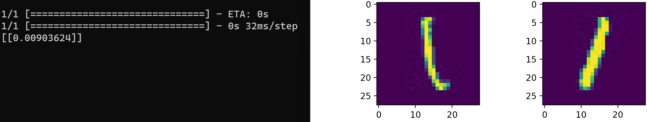
图8 图片相似度比较