Tensorflow2.1.0 Keras实现MNIST分类学习

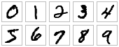
MNIST为手写数字图片集

代码

# 导入tensorflow库
import tensorflow as tf
# 导入os库
import os
# 从tensorflow中导入keras高级神经网络API
from tensorflow import keras
# 从keras中导入层，优化器，数据库，评估
from tensorflow.keras import layers, optimizers, datasets, metrics

# 从keras内置模型库中导入MNIST数据
(x_train, y_train),(x_test, y_test) = datasets.mnist.load_data()
# 将数据处理为[-1,1]之间，方便运算。 x_train的shape为（60000,28,28）
x_train = 2*tf.convert_to_tensor(x_train, dtype=tf.float32)/255. - 1

# 将x_train,y_train组合成一个数据集，方便运算
dateset = tf.data.Dataset.from_tensor_slices((x_train, y_train))
# 该数据训练集每次的训练数据batch为100，重复训练2次，根据情况修改参数
dateset = dateset.batch(100).repeat(2)

# 通过tf的张量创建训练模型，下面给出通过keras创建训练模型的代码，有兴趣可以试一下
'''
# Sequentital为keras下的创建线性叠加层的模块，利用该模块我们可以方便的搭建多层线性叠加
# layers.Dense创建全连接层，256为该连接层的输出，activation为该连接层输出时设置的激活哦函数
# 共设置了三层全连接层
model = keras.Sequential([layers.Dense(256, activation='relu'),
                     layers.Dense(128, activation='relu'),
                     layers.Dense(10)])
# 修改模型输入的shape
model.build(input_shape=(None,28*28))
model.summary()
'''
w1 = tf.Variable(tf.random.truncated_normal([784, 256], stddev=0.1))
b1 = tf.Variable(tf.zeros([256]))

w2 = tf.Variable(tf.random.truncated_normal([256,128], stddev=0.1))
b2 = tf.Variable(tf.zeros([128]))

w3 = tf.Variable(tf.random.truncated_normal([128,10], stddev=0.1))
b3 = tf.Variable(tf.zeros([10]))

variables = [w1, b1, w2, b2, w3, b3]

# 使用随机梯度模型优化器，学习率设置为0.001
optimizer = tf.keras.optimizers.SGD(learning_rate=1e-3)
# acc_meter为Keras模型评估metrics下的计算准确度的类
acc_meter = metrics.Accuracy()
for step, (x, y) in enumerate(dateset):
    with tf.GradientTape() as tape:
        x = tf.reshape(x, [-1, 28*28])
        h1 = x @ w1 + b1
        h1 = tf.nn.relu(h1)

        h2 = h1 @ w2 + b2
        h2 = tf.nn.relu(h2)

        out = h2 @ w3 + b3

        y_onehot = tf.one_hot(y, depth=10)

        loss = tf.reduce_mean(tf.square(out-y_onehot))

    # 计算并更新当前的准确率
    acc_meter.update_state(tf.argmax(out, axis=1), y)
    # 计算损失函数对模型参数的求导结果
    grads = tape.gradient(loss, variables)
    # 根据求导结果更新模型参数，从而使损失函数loss达到最小
    optimizer.apply_gradients(grads_and_vars=zip(grads, variables))

    #输出训练结果
    if step % 200 == 0:
        print(step, 'loss:', float(loss), 'acc:', acc_meter.result().numpy())
        acc_meter.reset_states()

计算结果

0 loss: 1.5610839128494263 acc: 0.12
200 loss: 0.40880781412124634 acc: 0.18175
400 loss: 0.23622004687786102 acc: 0.23715
600 loss: 0.17493964731693268 acc: 0.2914
800 loss: 0.22151599824428558 acc: 0.32865
1000 loss: 0.15884260833263397 acc: 0.35545