tensorflow学习（7. GAN实现MNIST分类）

https://blog.csdn.net/CoderPai/article/details/70598403?utm_source=blogxgwz0

里面有比较全面的GAN的链接

原始论文链接：http://papers.nips.cc/paper/5423-generative-adversarial-nets.pdf

一篇不错的理解GAN的文章：https://blog.csdn.net/qq_31531635/article/details/70670271

这篇GAN代码的出处 https://wiseodd.github.io/techblog/2016/09/17/gan-tensorflow/

简单用了别人的代码，实现了一下，加入了自己理解的部分：

import tensorflow as tf
import numpy as np
import matplotlib.pyplot as plt
import matplotlib.gridspec as gridspec
import os
from tensorflow.examples.tutorials.mnist import input_data

sess = tf.InteractiveSession()

mb_size = 128
Z_dim = 100

mnist = input_data.read_data_sets('../../MNIST_data', one_hot=True)

def weight_var(shape, name):
    return tf.get_variable(name=name, shape=shape, initializer=tf.contrib.layers.xavier_initializer())


def bias_var(shape, name):
    return tf.get_variable(name=name, shape=shape, initializer=tf.constant_initializer(0))


# discriminater net
#普通的两层卷积网络，作为鉴别网络
X = tf.placeholder(tf.float32, shape=[None, 784], name='X')

D_W1 = weight_var([784, 128], 'D_W1')
D_b1 = bias_var([128], 'D_b1')

D_W2 = weight_var([128, 1], 'D_W2')
D_b2 = bias_var([1], 'D_b2')


theta_D = [D_W1, D_W2, D_b1, D_b2]


# generator net
# 两层网络，输入为100维的噪声，这里是[-1,1]的均匀噪声，作为生成网络
Z = tf.placeholder(tf.float32, shape=[None, 100], name='Z')

G_W1 = weight_var([100, 128], 'G_W1')
G_b1 = bias_var([128], 'G_B1')

G_W2 = weight_var([128, 784], 'G_W2')
G_b2 = bias_var([784], 'G_B2')

theta_G = [G_W1, G_W2, G_b1, G_b2]

#具体网络的结构

def generator(z):
    G_h1 = tf.nn.relu(tf.matmul(z, G_W1) + G_b1)
    G_log_prob = tf.matmul(G_h1, G_W2) + G_b2
    G_prob = tf.nn.sigmoid(G_log_prob) #使用sigmoid给出该位置的值

    return G_prob


def discriminator(x):
    D_h1 = tf.nn.relu(tf.matmul(x, D_W1) + D_b1)
    D_logit = tf.matmul(D_h1, D_W2) + D_b2
    D_prob = tf.nn.sigmoid(D_logit) #使用sigmoid给出该位置的值
    return D_prob, D_logit

G_sample = generator(Z)
#X为实际的样本数据，G_sample为生成的样本数据
D_real, D_logit_real = discriminator(X)
D_fake, D_logit_fake = discriminator(G_sample)
'''
D_loss = -tf.reduce_mean(tf.log(D_real) + tf.log(1. - D_fake))
G_loss = -tf.reduce_mean(tf.log(D_fake))
'''
#D为辨别器，G为生成器，这里G是有助于辨别器提高性能的，G的输入是随机噪声，如果G没有训练，产出的应该是无关样本
#虽然也会提高一点性能，但是肯定不好，这里是希望G可以将噪声映射到合理的数字图的空间上，这里希望产出应该很接近
#合理图片，那么D很有可能被判别图像为真实图像，所以G_loss最小化对应为G_sample被D网络认定成真实图像
D_loss_real = tf.reduce_mean(tf.nn.sigmoid_cross_entropy_with_logits(
    logits=D_logit_real, labels=tf.ones_like(D_logit_real)))
D_loss_fake = tf.reduce_mean(tf.nn.sigmoid_cross_entropy_with_logits(
    logits=D_logit_fake, labels=tf.zeros_like(D_logit_fake)))
D_loss = D_loss_real + D_loss_fake
G_loss = tf.reduce_mean(tf.nn.sigmoid_cross_entropy_with_logits(
    logits=D_logit_fake, labels=tf.ones_like(D_logit_fake)))

#D和G还是比较独立的两部分，分别写开，不过两部分需要互相提高，所以后续的训练应该是交替进行
D_optimizer = tf.train.AdamOptimizer().minimize(D_loss, var_list=theta_D)
G_optimizer = tf.train.AdamOptimizer().minimize(G_loss, var_list=theta_G)
#随机数生成
def sample_Z(m, n):
    '''Uniform prior for G(Z)'''
    return np.random.uniform(-1., 1., size=[m, n])


def plot(samples):
    fig = plt.figure(figsize=(4, 4))
    gs = gridspec.GridSpec(4, 4)
    gs.update(wspace=0.05, hspace=0.05)

    for i, sample in enumerate(samples):  # [i,samples[i]] imax=16
        ax = plt.subplot(gs[i])
        plt.axis('off')
        ax.set_xticklabels([])
        ax.set_aspect('equal')
        plt.imshow(sample.reshape(28, 28), cmap='Greys_r')

    return fig



if not os.path.exists('out/'):
    os.makedirs('out/')

sess.run(tf.global_variables_initializer())

i = 0
for it in range(1000000):
    #每1000次输出一次
    if it % 1000 == 0:
        samples = sess.run(G_sample, feed_dict={
                           Z: sample_Z(16, Z_dim)})  # 16*784
        fig = plot(samples)
        #图像存储
        plt.savefig('out/{}.png'.format(str(i).zfill(3)), bbox_inches='tight')
        i += 1
        plt.close(fig)

    X_mb, _ = mnist.train.next_batch(mb_size)
    #D和G的交替训练，进行性能的互相提高
    _, D_loss_curr = sess.run([D_optimizer, D_loss], feed_dict={
                              X: X_mb, Z: sample_Z(mb_size, Z_dim)})
    _, G_loss_curr = sess.run([G_optimizer, G_loss], feed_dict={
                              Z: sample_Z(mb_size, Z_dim)})

    if it % 1000 == 0:
        print('Iter: {}'.format(it))
        print('D loss: {:.4}'.format(D_loss_curr))
        print('G_loss: {:.4}'.format(G_loss_curr))
        print()

运行的结果是每1000次生成的图像，前200张做成了视频，结果如下：

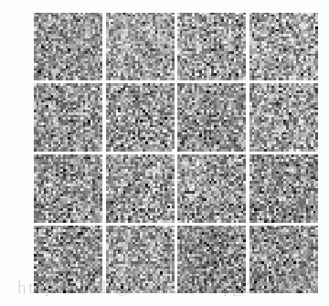
总结一下：

1.GAN还是一种解决问题的框架，通过生成网络G产生更高相关度的图像来提升判别网络D的性能

2.本文方法仅仅使用了神经网络，没有使用CNN，使用CNN产生判别网络才是更合适的，本文在产生的200张的动图后半部分图像变化不明显，将Loss显示出来也可以看出来结果提升不高，这是网络结构较差的原因。

3.GAN不止是提高判别网络D的性能，也可以通过GAN的生成网络G产生平价数据（弱监督中，有标签数据较少，无标签数据较多的情形)。可以通过GAN的生成网络产生更多的有标签数据用于训练，论文见SSGAN。博客链接：https://blog.csdn.net/shenxiaolu1984/article/details/75736407

之后要看的一些东西：

1.Fine-tunning，复用别人的网络并进行新的应用开发，学习网址链接：https://blog.csdn.net/u011600477/article/details/78607883

2.RCNN，博客见：https://blog.csdn.net/v1_vivian/article/details/78599229?utm_source=blogxgwz0，https://blog.csdn.net/WoPawn/article/details/52133338。RCNN关键在于预搜索框的选取，论文是Selective Search for Object Recognition，博客链接：https://blog.csdn.net/surgewong/article/details/39316931

3.YOLO: You Only Look Once，和RCNN的功能一致，但是想法不同，博客：https://blog.csdn.net/shenxiaolu1984/article/details/78826995

4.可视化网络结构特征

tensorflow学习（7. GAN实现MNIST分类）

猜你喜欢