粒子滤波器(Particle Filter)
概念
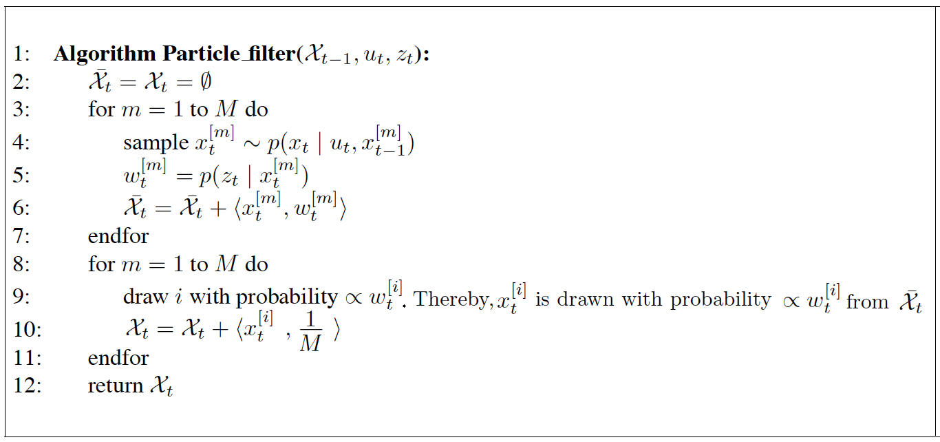
(来源:Probabilistic Robotics, 4.3 The Particle Filter, p96)
解析:
- line 3 - 7: 生成M个新样本(即粒子)
- line 4: 根据重要性(importance weight)采样
- line 5: (重新)计算重要性(re-weight)
- line 6: 更新标准化(update normalization)准确翻译待确认
- line 8 -11: 重采样(resampling or importance sampling)
- line 9:
- line 10:
比喻
待补充
示例程序
"""

Particle Filter localization sample

author: Atsushi Sakai (@Atsushi_twi)

"""

import math

import matplotlib.pyplot as plt
import numpy as np

# Estimation parameter of PF
Q = np.diag([0.2]) ** 2  # range error
R = np.diag([2.0, np.deg2rad(40.0)]) ** 2  # input error

#  Simulation parameter
Q_sim = np.diag([0.2]) ** 2
R_sim = np.diag([1.0, np.deg2rad(30.0)]) ** 2

DT = 0.1  # time tick [s]
SIM_TIME = 50.0  # simulation time [s]
MAX_RANGE = 20.0  # maximum observation range

# Particle filter parameter
NP = 100  # Number of Particle
NTh = NP / 2.0  # Number of particle for re-sampling

show_animation = True


def calc_input():
    v = 1.0  # [m/s]
    yaw_rate = 0.1  # [rad/s]
    u = np.array([[v, yaw_rate]]).T
    return u


def observation(x_true, xd, u, rf_id):
    x_true = motion_model(x_true, u)

    # add noise to gps x-y
    z = np.zeros((0, 3))

    for i in range(len(rf_id[:, 0])):

        dx = x_true[0, 0] - rf_id[i, 0]
        dy = x_true[1, 0] - rf_id[i, 1]
        d = math.hypot(dx, dy)
        if d <= MAX_RANGE:
            dn = d + np.random.randn() * Q_sim[0, 0] ** 0.5  # add noise
            zi = np.array([[dn, rf_id[i, 0], rf_id[i, 1]]])
            z = np.vstack((z, zi))

    # add noise to input
    ud1 = u[0, 0] + np.random.randn() * R_sim[0, 0] ** 0.5
    ud2 = u[1, 0] + np.random.randn() * R_sim[1, 1] ** 0.5
    ud = np.array([[ud1, ud2]]).T

    xd = motion_model(xd, ud)

    return x_true, z, xd, ud


def motion_model(x, u):
    F = np.array([[1.0, 0, 0, 0],
                  [0, 1.0, 0, 0],
                  [0, 0, 1.0, 0],
                  [0, 0, 0, 0]])

    B = np.array([[DT * math.cos(x[2, 0]), 0],
                  [DT * math.sin(x[2, 0]), 0],
                  [0.0, DT],
                  [1.0, 0.0]])

    x = F.dot(x) + B.dot(u)

    return x


def gauss_likelihood(x, sigma):
    p = 1.0 / math.sqrt(2.0 * math.pi * sigma ** 2) * \
        math.exp(-x ** 2 / (2 * sigma ** 2))

    return p


def calc_covariance(x_est, px, pw):
    """
    calculate covariance matrix
    see ipynb doc
    """
    cov = np.zeros((3, 3))
    n_particle = px.shape[1]
    for i in range(n_particle):
        dx = (px[:, i:i + 1] - x_est)[0:3]
        cov += pw[0, i] * dx @ dx.T
    cov *= 1.0 / (1.0 - pw @ pw.T)

    return cov


def pf_localization(px, pw, z, u):
    """
    Localization with Particle filter
    """

    for ip in range(NP):
        x = np.array([px[:, ip]]).T
        w = pw[0, ip]

        #  Predict with random input sampling
        ud1 = u[0, 0] + np.random.randn() * R[0, 0] ** 0.5
        ud2 = u[1, 0] + np.random.randn() * R[1, 1] ** 0.5
        ud = np.array([[ud1, ud2]]).T
        x = motion_model(x, ud)

        #  Calc Importance Weight
        for i in range(len(z[:, 0])):
            dx = x[0, 0] - z[i, 1]
            dy = x[1, 0] - z[i, 2]
            pre_z = math.hypot(dx, dy)
            dz = pre_z - z[i, 0]
            w = w * gauss_likelihood(dz, math.sqrt(Q[0, 0]))

        px[:, ip] = x[:, 0]
        pw[0, ip] = w

    pw = pw / pw.sum()  # normalize

    x_est = px.dot(pw.T)
    p_est = calc_covariance(x_est, px, pw)

    N_eff = 1.0 / (pw.dot(pw.T))[0, 0]  # Effective particle number
    if N_eff < NTh:
        px, pw = re_sampling(px, pw)
    return x_est, p_est, px, pw


def re_sampling(px, pw):
    """
    low variance re-sampling
    """

    w_cum = np.cumsum(pw)
    base = np.arange(0.0, 1.0, 1 / NP)
    re_sample_id = base + np.random.uniform(0, 1 / NP)
    indexes = []
    ind = 0
    for ip in range(NP):
        while re_sample_id[ip] > w_cum[ind]:
            ind += 1
        indexes.append(ind)

    px = px[:, indexes]
    pw = np.zeros((1, NP)) + 1.0 / NP  # init weight

    return px, pw


def plot_covariance_ellipse(x_est, p_est):  # pragma: no cover
    p_xy = p_est[0:2, 0:2]
    eig_val, eig_vec = np.linalg.eig(p_xy)

    if eig_val[0] >= eig_val[1]:
        big_ind = 0
        small_ind = 1
    else:
        big_ind = 1
        small_ind = 0

    t = np.arange(0, 2 * math.pi + 0.1, 0.1)

    # eig_val[big_ind] or eiq_val[small_ind] were occasionally negative numbers extremely
    # close to 0 (~10^-20), catch these cases and set the respective variable to 0
    try:
        a = math.sqrt(eig_val[big_ind])
    except ValueError:
        a = 0

    try:
        b = math.sqrt(eig_val[small_ind])
    except ValueError:
        b = 0

    x = [a * math.cos(it) for it in t]
    y = [b * math.sin(it) for it in t]
    angle = math.atan2(eig_vec[big_ind, 1], eig_vec[big_ind, 0])
    Rot = np.array([[math.cos(angle), -math.sin(angle)],
                    [math.sin(angle), math.cos(angle)]])
    fx = Rot.dot(np.array([[x, y]]))
    px = np.array(fx[0, :] + x_est[0, 0]).flatten()
    py = np.array(fx[1, :] + x_est[1, 0]).flatten()
    plt.plot(px, py, "--r")


def main():
    print(__file__ + " start!!")

    time = 0.0

    # RF_ID positions [x, y]
    rf_id = np.array([[10.0, 0.0],
                      [10.0, 10.0],
                      [0.0, 15.0],
                      [-5.0, 20.0]])

    # State Vector [x y yaw v]'
    x_est = np.zeros((4, 1))
    x_true = np.zeros((4, 1))

    px = np.zeros((4, NP))  # Particle store
    pw = np.zeros((1, NP)) + 1.0 / NP  # Particle weight
    x_dr = np.zeros((4, 1))  # Dead reckoning

    # history
    h_x_est = x_est
    h_x_true = x_true
    h_x_dr = x_true

    while SIM_TIME >= time:
        time += DT
        u = calc_input()

        x_true, z, x_dr, ud = observation(x_true, x_dr, u, rf_id)

        x_est, PEst, px, pw = pf_localization(px, pw, z, ud)

        # store data history
        h_x_est = np.hstack((h_x_est, x_est))
        h_x_dr = np.hstack((h_x_dr, x_dr))
        h_x_true = np.hstack((h_x_true, x_true))

        if show_animation:
            plt.cla()
            # for stopping simulation with the esc key.
            plt.gcf().canvas.mpl_connect('key_release_event',
                                         lambda event: [exit(0) if event.key == 'escape' else None])

            for i in range(len(z[:, 0])):
                plt.plot([x_true[0, 0], z[i, 1]], [x_true[1, 0], z[i, 2]], "-k")
            plt.plot(rf_id[:, 0], rf_id[:, 1], "*k")
            plt.plot(px[0, :], px[1, :], ".r")
            plt.plot(np.array(h_x_true[0, :]).flatten(),
                     np.array(h_x_true[1, :]).flatten(), "-b")
            plt.plot(np.array(h_x_dr[0, :]).flatten(),
                     np.array(h_x_dr[1, :]).flatten(), "-k")
            plt.plot(np.array(h_x_est[0, :]).flatten(),
                     np.array(h_x_est[1, :]).flatten(), "-r")
            plot_covariance_ellipse(x_est, PEst)
            plt.axis("equal")
            plt.grid(True)
            plt.pause(0.001)


if __name__ == '__main__':
    main()
核心代码
def pf_localization(px, pw, z, u):
    """
    Localization with Particle filter
    """

    for ip in range(NP):
        x = np.array([px[:, ip]]).T
        w = pw[0, ip]

        #  Predict with random input sampling
        ud1 = u[0, 0] + np.random.randn() * R[0, 0] ** 0.5
        ud2 = u[1, 0] + np.random.randn() * R[1, 1] ** 0.5
        ud = np.array([[ud1, ud2]]).T
        x = motion_model(x, ud)

        #  Calc Importance Weight
        for i in range(len(z[:, 0])):
            dx = x[0, 0] - z[i, 1]
            dy = x[1, 0] - z[i, 2]
            pre_z = math.hypot(dx, dy)
            dz = pre_z - z[i, 0]
            w = w * gauss_likelihood(dz, math.sqrt(Q[0, 0]))

        px[:, ip] = x[:, 0]
        pw[0, ip] = w

    pw = pw / pw.sum()  # normalize

    x_est = px.dot(pw.T)
    p_est = calc_covariance(x_est, px, pw)

    N_eff = 1.0 / (pw.dot(pw.T))[0, 0]  # Effective particle number
    if N_eff < NTh:
        px, pw = re_sampling(px, pw)
    return x_est, p_est, px, pw
步骤1:初始化
    px = np.zeros((4, NP))  # Particle store
    pw = np.zeros((1, NP)) + 1.0 / NP  # Particle weight
步骤2:采样
    for ip in range(NP):
        x = np.array([px[:, ip]]).T
        w = pw[0, ip]

        #  Predict with random input sampling
        ud1 = u[0, 0] + np.random.randn() * R[0, 0] ** 0.5
        ud2 = u[1, 0] + np.random.randn() * R[1, 1] ** 0.5
        ud = np.array([[ud1, ud2]]).T
        x = motion_model(x, ud)

        #  Calc Importance Weight
        for i in range(len(z[:, 0])):
            dx = x[0, 0] - z[i, 1]
            dy = x[1, 0] - z[i, 2]
            pre_z = math.hypot(dx, dy)
            dz = pre_z - z[i, 0]
            w = w * gauss_likelihood(dz, math.sqrt(Q[0, 0]))

        px[:, ip] = x[:, 0]
        pw[0, ip] = w

    pw = pw / pw.sum()  # normalize
1)基于模型预测粒子状态:
        #  Predict with random input sampling
        ud1 = u[0, 0] + np.random.randn() * R[0, 0] ** 0.5
        ud2 = u[1, 0] + np.random.randn() * R[1, 1] ** 0.5
        ud = np.array([[ud1, ud2]]).T
x = motion_model(x, ud)2)计算重要性权重:这部分还有点懵
        #  Calc Importance Weight
        for i in range(len(z[:, 0])):
            dx = x[0, 0] - z[i, 1]
            dy = x[1, 0] - z[i, 2]
            pre_z = math.hypot(dx, dy)
            dz = pre_z - z[i, 0]
            w = w * gauss_likelihood(dz, math.sqrt(Q[0, 0]))
dz = pre_z - z[i, 0]得到的是到地标i距离先验和后验的差别,直觉上理解,与实际值(先验)差别越大,说明该测量值(后验)越不可信,也就是权重越低,与之前的权重w累乘w = w * gauss_likelihood(dz, math.sqrt(Q[0, 0])),那么会得到新的权重值。
步骤3:重采样
    if N_eff < NTh:
        px, pw = re_sampling(px, pw)
参考
- https://en.wikipedia.org/wiki/Particle_filter
- Probabilistic Robotics, 4.3 The Particle Filter, p96-113
- Coursera: Robotics-Estimation-and-Learning, Course5-Estimation-and-Learning: AssignmentWEEK4