tensorflow学习笔记 + 程序 (五)CNN与MNIST数据集

下文中所用的部分数据集链接(百度网盘):
链接：https://pan.baidu.com/s/1_Y0rWLj9wuJefzT9JME5Ug
提取码：6fho

1 基础CNN用于MNIST

1.1 部分函数介绍

1.1.1 tf.nn.conv2d

tf.nn.conv2d(input, filter, strides, padding, use_cudnn_on_gpu=None, name=None)

第一个参数input：指需要做卷积的输入图像，它要求是一个Tensor，具有[batch, in_height, in_width, in_channels]这样的shape，具体含义是[训练时一个batch的图片数量, 图片高度, 图片宽度, 图像通道数]，注意这是一个4维的Tensor，要求类型为float32和float64其中之一

第二个参数filter：相当于CNN中的卷积核，它要求是一个Tensor，具有[filter_height, filter_width, in_channels, out_channels]这样的shape，具体含义是[卷积核的高度，卷积核的宽度，图像通道数，卷积核个数]，要求类型与参数input相同，有一个地方需要注意，第三维in_channels，就是参数input的第四维

第三个参数strides：卷积时在图像每一维的步长，这是一个一维的向量，长度4

第四个参数padding：string类型的量，只能是"SAME","VALID"其中之一，这个值决定了不同的卷积方式，(SAME表示添加全0填充，VALID表示不添加)

第五个参数：use_cudnn_on_gpu:bool类型，是否使用cudnn加速，默认为true

参考链接 : 【TensorFlow】tf.nn.conv2d是怎样实现卷积的？

1.1.2 tf.nn.max_pool

tf.nn.max_pool(h,ksize=[1, height, width, 1],strides=[1, 1, 1, 1],padding='VALID',name="pool")

第一个参数h : 需要池化的输入，一般池化层接在卷积层后面，所以输入通常是feature map，依然是[batch_size, height, width, channels]这样的shape
第二个参数k_size : 池化窗口的大小，取一个四维向量，一般是[1, height, width, 1]，因为我们不想在batch和channels上做池化，所以这两个维度设为了1
第三个参数strides : 窗口在每一个维度上滑动的步长，一般也是[1, stride,stride, 1]
第四个参数padding： 填充的方法，SAME或VALID，SAME表示添加全0填充，VALID表示不添加
第五个参数name(命名)就是你给它起个名字，然后tensorboard流程图里能看见
.上面那个name也是这样

参考链接 : tf.nn.max_pool函数详解

1.1.3 tf.truncated_normal

tf.truncated_normal(shape, mean=0.0, stddev=1.0, dtype=tf.float32, seed=None, name=None)

第一个参数shape: 一维的张量，也是输出的张量。
第二个参数mean: 正态分布的均值。
第三个参数stddev: 正态分布的标准差。
第四个参数dtype: 输出的类型。
第五个参数seed: 一个整数，当设置之后，每次生成的随机数都一样。

参考链接 : tf.truncated_normal

1.2 完整程序

import tensorflow as tf
from tensorflow.examples.tutorials.mnist import input_data

# 载入数据集
mnist = input_data.read_data_sets("MNIST_data",one_hot=True)

# 每个批次的大小
batch_size = 100
# 计算一共有多少个批次
n_batch = mnist.train.num_examples // batch_size

# 权值初始化
def weight_variable(shape):
    initial = tf.truncated_normal(shape,stddev=0.1)
    # 生成一个截断的正态分布,其标准差为0.1
    return tf.Variable(initial)

# 偏置初始化 
def bias_variable(shape):
    initial = tf.constant(0.1,shape=shape)
    return tf.Variable(initial)

# 卷积层
def conv2d(x,W):
    return tf.nn.conv2d(x,W,strides=[1,1,1,1],padding="SAME") 
    # x为输入的tensor,其形状为[batch, in_height, in_width, in_channels],具体含义是[训练时一个batch的图片数量, 图片高度, 图片宽度, 图像通道数]
    # W为卷积核(滤波器),其形状为[filter_height, filter_width, in_channels, out_channels],具体含义是[卷积核的高度，卷积核的宽度，图像通道数，卷积核个数]
    # strides[0]和strides[3]的两个1是默认值,strides[1]代表x方向的步长，strides[2]代表y方向的步长
    # padding决定卷积方式,SAME会在外面补0

# 池化层(最大值池化)
def max_pool_2x2(x):
    return tf.nn.max_pool(x,ksize=[1,2,2,1],strides=[1,2,2,1],padding="SAME")
    # ksize[0]和ksize[3]默认为1,中间的2,2为池化窗口的大小
    # strides同conv2d,明显x,y方向的步长均为2

# 定义两个placeholder
x = tf.placeholder(tf.float32,[None,784])
y = tf.placeholder(tf.float32,[None,10])

# 改变x格式为4D的向量
x_image = tf.reshape(x,[-1,28,28,1]) 
# 第二个参数 : [batch, in_height, in_width, in_channels] [训练时一个batch的图片数量, 图片高度, 图片宽度, 图像通道数]
# 其中-1在程序运行后将会被赋值为100(即每批次中包含的图片的数量)

# 初始化第一个卷积层的权值和偏置
W_conv1 = weight_variable([5,5,1,32]) 
# 5*5的采样窗口,32个卷积核(32个平面/32个通道)从一个平面(一个通道)提取特征
b_conv1 = bias_variable([32]) 
# 每一个卷积核一个偏置值

# 把x_image和权值向量进行卷积,再加上偏置值,并用relu激活函数
h_conv1 = tf.nn.relu(conv2d(x_image,W_conv1) + b_conv1)
# x_image和W_conv1进行2D卷积操作再加上权值,最后输入relu激活函数

# 将第一卷积层输出进行池化
h_pool1 = max_pool_2x2(h_conv1)

# 初始化第二个卷积层的权值和偏置
W_conv2 = weight_variable([5,5,32,64]) # 5*5的采样窗口,64个卷积核从32个平面提取特征
b_conv2 = bias_variable([64]) # 每一个卷积核一个偏置值

# 把h_pool1和权值向量进行卷积,再加上偏置值,并用relu激活函数
h_conv2 = tf.nn.relu(conv2d(h_pool1,W_conv2) + b_conv2)

# 将第二卷积层输出进行池化
h_pool2 = max_pool_2x2(h_conv2)

# 说下这些卷积池化的过程(数据形状) : 
#   28*28的图片第一次卷积后还是28*28(SAME padding不会改变图片的大小),第一次池化后变为14*14
#   14*14的图片第二次卷积后还是14*14,第二次池化后变为7*7
#   经上述操作后最后获得64张7*7平面

# 初始化第一个全连接层的权值
W_fc1 = weight_variable([7*7*64,1024]) 
# 上一层共有7*7*64个像素点,全连接层1共1024个神经元
b_fc1 = bias_variable([1024])
# 每个神经元一个偏置值

# 把池化层2的输出扁平化为1维
h_pool2_flat = tf.reshape(h_pool2,[-1,7*7*64])
# h_pool2为形状为[100(批次),7,7(高宽),64(图片或者通道数)]
# -1为任意值,计算时会处理为100
# 实际上就是将其后三个维度转化为7*7*64这一个维度

# 求第一个全连接层的输出
h_fc1 = tf.nn.relu(tf.matmul(h_pool2_flat,W_fc1) + b_fc1) 

# 用keep_prob来表示神经元的输出概率(dropout)
keep_prob = tf.placeholder(tf.float32)
h_fc1_drop = tf.nn.dropout(h_fc1,keep_prob)

# 初始化第二个全连接层
W_fc2 = weight_variable([1024,10])
b_fc2 = bias_variable([10])

# 计算输出
prediction = tf.nn.softmax(tf.matmul(h_fc1_drop,W_fc2) + b_fc2)

# 交叉熵代价函数
cross_entropy = tf.reduce_mean(tf.nn.softmax_cross_entropy_with_logits(labels=y,logits=prediction))
# 使用AdamOptimizer进行优化
train_step = tf.train.AdamOptimizer(1e-4).minimize(cross_entropy)
# 结果存放在一个bool型列表中
correct_prediction = tf.equal(tf.argmax(prediction,1),tf.argmax(y,1)) # argmax返回一维张量中最大值所在的位置
# 求准确率
accuracy = tf.reduce_mean(tf.cast(correct_prediction,tf.float32))

with tf.Session() as sess:
    sess.run(tf.global_variables_initializer())
    for epoch in range(21):
        for batch in range(n_batch):
            # 传入数据
            batch_xs,batch_ys =  mnist.train.next_batch(batch_size)
            # 用70%的神经元训练网络(dropout)
            sess.run(train_step,feed_dict={x:batch_xs,y:batch_ys,keep_prob:0.7})

        # 运行100%的神经元来检测网络准确率
        acc = sess.run(accuracy,feed_dict={x:mnist.test.images,y:mnist.test.labels,keep_prob:1.0})
        # 输出
        print ("Iter " + str(epoch) + ", Testing Accuracy= " + str(acc))


# 输出结果
'''
Iter 0, Testing Accuracy= 0.9529
Iter 1, Testing Accuracy= 0.9723
Iter 2, Testing Accuracy= 0.9785
Iter 3, Testing Accuracy= 0.9818
Iter 4, Testing Accuracy= 0.985
Iter 5, Testing Accuracy= 0.9859
Iter 6, Testing Accuracy= 0.9871
Iter 7, Testing Accuracy= 0.9896
Iter 8, Testing Accuracy= 0.9874
Iter 9, Testing Accuracy= 0.9899
Iter 10, Testing Accuracy= 0.9893
Iter 11, Testing Accuracy= 0.9901
Iter 12, Testing Accuracy= 0.9905
Iter 13, Testing Accuracy= 0.9899
Iter 14, Testing Accuracy= 0.9908
Iter 15, Testing Accuracy= 0.9913
Iter 16, Testing Accuracy= 0.991
Iter 17, Testing Accuracy= 0.9907
Iter 18, Testing Accuracy= 0.9917
Iter 19, Testing Accuracy= 0.9917
Iter 20, Testing Accuracy= 0.9917
'''

多说两句,一是一般情况下池化层并不单算一层,其往往算作卷积层的附属
二是现在池化层并不是很受青睐。部分原因是：池化导致信息损失,还可能导致欠拟合问题

2 CNN可视化

2.1 程序

import tensorflow as tf
from tensorflow.examples.tutorials.mnist import input_data

# 载入数据集
mnist = input_data.read_data_sets('MNIST_data',one_hot=True)

# 每个批次的大小
batch_size = 100
# 计算一共有多少个批次
n_batch = mnist.train.num_examples // batch_size

# 参数概要(拿过来是拿过来了,不过貌似没用上)
def variable_summaries(var):
    with tf.name_scope('summaries'):
        mean = tf.reduce_mean(var)
        tf.summary.scalar('mean', mean) # 平均值
        with tf.name_scope('stddev'):
            stddev = tf.sqrt(tf.reduce_mean(tf.square(var - mean)))
        tf.summary.scalar('stddev', stddev) # 标准差
        tf.summary.scalar('max', tf.reduce_max(var)) # 最大值
        tf.summary.scalar('min', tf.reduce_min(var) )# 最小值
        tf.summary.histogram('histogram', var) # 直方图

# 初始化权值
def weight_variable(shape,name):
    initial = tf.truncated_normal(shape,stddev=0.1)
    # 生成一个截断的正态分布
    return tf.Variable(initial,name=name)

# 初始化偏置
def bias_variable(shape,name):
    initial = tf.constant(0.1,shape=shape)
    return tf.Variable(initial,name=name)

# 卷积层
def conv2d(x,W):
    return tf.nn.conv2d(x,W,strides=[1,1,1,1],padding='SAME')

# 池化层
def max_pool_2x2(x):
    return tf.nn.max_pool(x,ksize=[1,2,2,1],strides=[1,2,2,1],padding='SAME')

# 命名空间
with tf.name_scope('input'):
    # 定义两个placeholder
    x = tf.placeholder(tf.float32,[None,784],name='x-input')
    y = tf.placeholder(tf.float32,[None,10],name='y-input')
    with tf.name_scope('x_image'):
        # 改变x的格式转为4D的向量[batch, in_height, in_width, in_channels]`
        x_image = tf.reshape(x,[-1,28,28,1],name='x_image')


with tf.name_scope('Conv1'):
    # 初始化第一个卷积层的权值和偏置
    with tf.name_scope('W_conv1'):
        W_conv1 = weight_variable([5,5,1,32],name='W_conv1')
        # 5*5的采样窗口，32个卷积核从1个平面抽取特征
    with tf.name_scope('b_conv1'):  
        b_conv1 = bias_variable([32],name='b_conv1')
        # 每一个卷积核一个偏置值

    # 把x_image和权值向量进行卷积，再加上偏置值，然后应用于relu激活函数
    with tf.name_scope('conv2d_1'):
        conv2d_1 = conv2d(x_image,W_conv1) + b_conv1
    with tf.name_scope('relu'):
        h_conv1 = tf.nn.relu(conv2d_1)
    with tf.name_scope('h_pool1'):
        h_pool1 = max_pool_2x2(h_conv1)
        # 进行max-pooling

with tf.name_scope('Conv2'):
    # 初始化第二个卷积层的权值和偏置
    with tf.name_scope('W_conv2'):
        W_conv2 = weight_variable([5,5,32,64],name='W_conv2')
        # 5*5的采样窗口，64个卷积核从32个平面抽取特征
    with tf.name_scope('b_conv2'):  
        b_conv2 = bias_variable([64],name='b_conv2')
        # 每一个卷积核一个偏置值

    # 把h_pool1和权值向量进行卷积，再加上偏置值，然后应用于relu激活函数
    with tf.name_scope('conv2d_2'):
        conv2d_2 = conv2d(h_pool1,W_conv2) + b_conv2
    with tf.name_scope('relu'):
        h_conv2 = tf.nn.relu(conv2d_2)
    with tf.name_scope('h_pool2'):
        h_pool2 = max_pool_2x2(h_conv2)
        # 进行max-pooling

with tf.name_scope('fc1'):
    # 初始化第一个全连接层的权值
    with tf.name_scope('W_fc1'):
        W_fc1 = weight_variable([7*7*64,1024],name='W_fc1')
        # 上一场有7*7*64个神经元，全连接层有1024个神经元
    with tf.name_scope('b_fc1'):
        b_fc1 = bias_variable([1024],name='b_fc1')
        # 1024个节点

    # 把池化层2的输出扁平化为1维
    with tf.name_scope('h_pool2_flat'):
        h_pool2_flat = tf.reshape(h_pool2,[-1,7*7*64],name='h_pool2_flat')

    # 求第一个全连接层的输出
    with tf.name_scope('wx_plus_b1'):
        wx_plus_b1 = tf.matmul(h_pool2_flat,W_fc1) + b_fc1
    with tf.name_scope('relu'):
        h_fc1 = tf.nn.relu(wx_plus_b1)

    # keep_prob用来表示神经元的输出概率
    with tf.name_scope('keep_prob'):
        keep_prob = tf.placeholder(tf.float32,name='keep_prob')
    with tf.name_scope('h_fc1_drop'):
        h_fc1_drop = tf.nn.dropout(h_fc1,keep_prob,name='h_fc1_drop')

with tf.name_scope('fc2'):
    # 初始化第二个全连接层
    with tf.name_scope('W_fc2'):
        W_fc2 = weight_variable([1024,10],name='W_fc2')
    with tf.name_scope('b_fc2'):    
        b_fc2 = bias_variable([10],name='b_fc2')
    with tf.name_scope('wx_plus_b2'):
        wx_plus_b2 = tf.matmul(h_fc1_drop,W_fc2) + b_fc2
    with tf.name_scope('softmax'):
        # 计算输出
        prediction = tf.nn.softmax(wx_plus_b2)

# 交叉熵代价函数
with tf.name_scope('cross_entropy'):
    cross_entropy = tf.reduce_mean(tf.nn.softmax_cross_entropy_with_logits(labels=y,logits=prediction),name='cross_entropy')
    # 
    tf.summary.scalar('cross_entropy',cross_entropy)
    
# 使用AdamOptimizer进行优化
with tf.name_scope('train'):
    train_step = tf.train.AdamOptimizer(1e-4).minimize(cross_entropy)

# 求准确率
with tf.name_scope('accuracy'):
    with tf.name_scope('correct_prediction'):
        # 结果存放在一个布尔列表中
        correct_prediction = tf.equal(tf.argmax(prediction,1),tf.argmax(y,1))#argmax返回一维张量中最大的值所在的位置
    with tf.name_scope('accuracy'):
        # 求准确率
        accuracy = tf.reduce_mean(tf.cast(correct_prediction,tf.float32))
        tf.summary.scalar('accuracy',accuracy)
        
# 合并所有的summary
merged = tf.summary.merge_all()

with tf.Session() as sess:
    sess.run(tf.global_variables_initializer())
    train_writer = tf.summary.FileWriter('logs/train',sess.graph)
    test_writer = tf.summary.FileWriter('logs/test',sess.graph)
    for i in range(1001):
        # 训练模型
        batch_xs,batch_ys =  mnist.train.next_batch(batch_size)
        sess.run(train_step,feed_dict={x:batch_xs,y:batch_ys,keep_prob:0.5})
        # 记录训练集计算的参数
        summary = sess.run(merged,feed_dict={x:batch_xs,y:batch_ys,keep_prob:1.0})
        train_writer.add_summary(summary,i)
        # 记录测试集计算的参数
        batch_xs,batch_ys =  mnist.test.next_batch(batch_size)
        summary = sess.run(merged,feed_dict={x:batch_xs,y:batch_ys,keep_prob:1.0})
        test_writer.add_summary(summary,i)
    
        if i%100==0:
            test_acc = sess.run(accuracy,feed_dict={x:mnist.test.images,y:mnist.test.labels,keep_prob:1.0})
            train_acc = sess.run(accuracy,feed_dict={x:mnist.train.images[:10000],y:mnist.train.labels[:10000],keep_prob:1.0})
            print ("Iter " + str(i) + ", Testing Accuracy= " + str(test_acc) + ", Training Accuracy= " + str(train_acc))


# 输出结果
'''
Iter 100, Testing Accuracy= 0.5381, Training Accuracy= 0.531
Iter 200, Testing Accuracy= 0.5675, Training Accuracy= 0.5604
Iter 300, Testing Accuracy= 0.5737, Training Accuracy= 0.5676
Iter 400, Testing Accuracy= 0.6662, Training Accuracy= 0.6616
Iter 500, Testing Accuracy= 0.6697, Training Accuracy= 0.6681
Iter 600, Testing Accuracy= 0.7902, Training Accuracy= 0.7972
Iter 700, Testing Accuracy= 0.8615, Training Accuracy= 0.8643
Iter 800, Testing Accuracy= 0.957, Training Accuracy= 0.9529
Iter 900, Testing Accuracy= 0.9581, Training Accuracy= 0.9563
Iter 1000, Testing Accuracy= 0.96, Training Accuracy= 0.9567
'''

方法详见我上一篇博客 : tensorflow学习笔记 + 程序 (四)tensorboard可视化

2.2 tensorboard

2.2.1 scalars

2.2.1.1 accuracy(准确率)

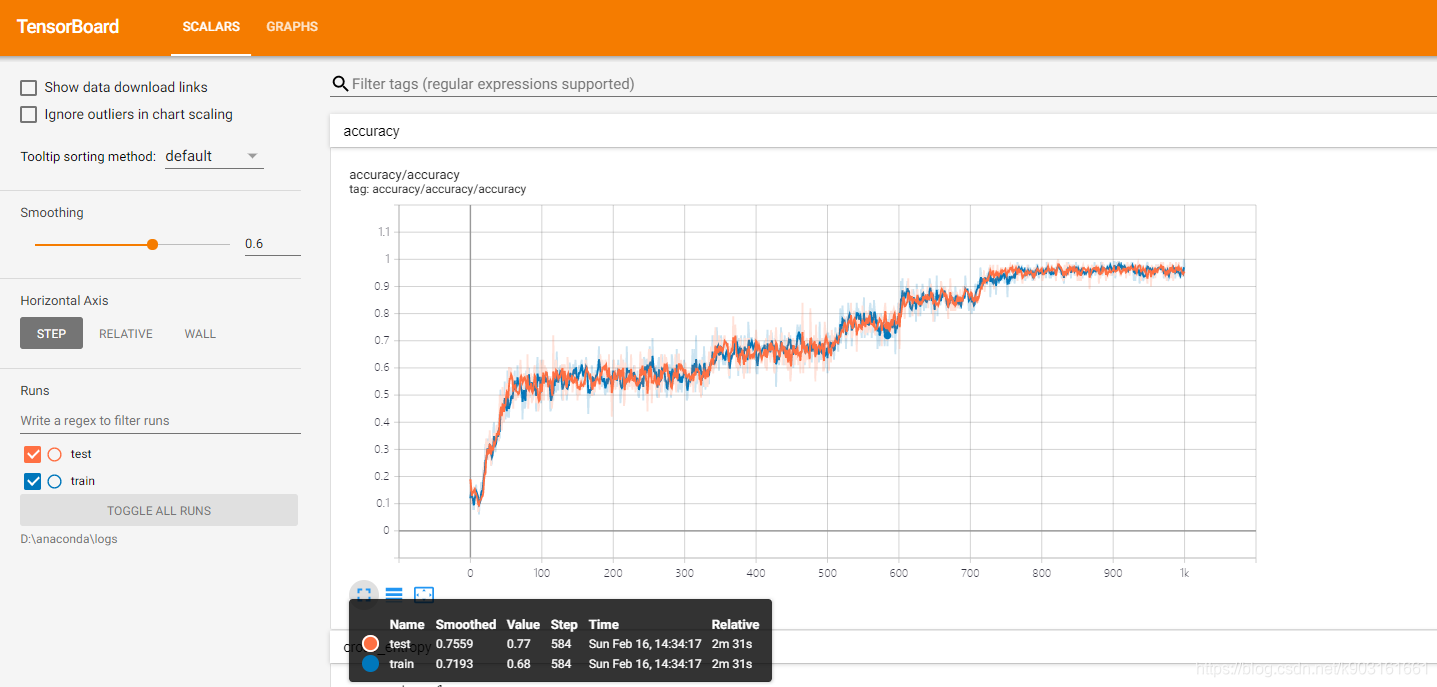
由于最后生成了两个文件一个为训练集一个为测试集,故而这里也就有两种颜色(橙色为测试集,蓝色为训练集),目前来看,这两条曲线比较接近,这说明这个模型既没有欠拟合的情况也没有过拟合的情况,模型训练的比较好,如果模型过拟合,则蓝色曲线应该高于橙色曲线,反之若为欠拟合,则橙色线应该略高于蓝色

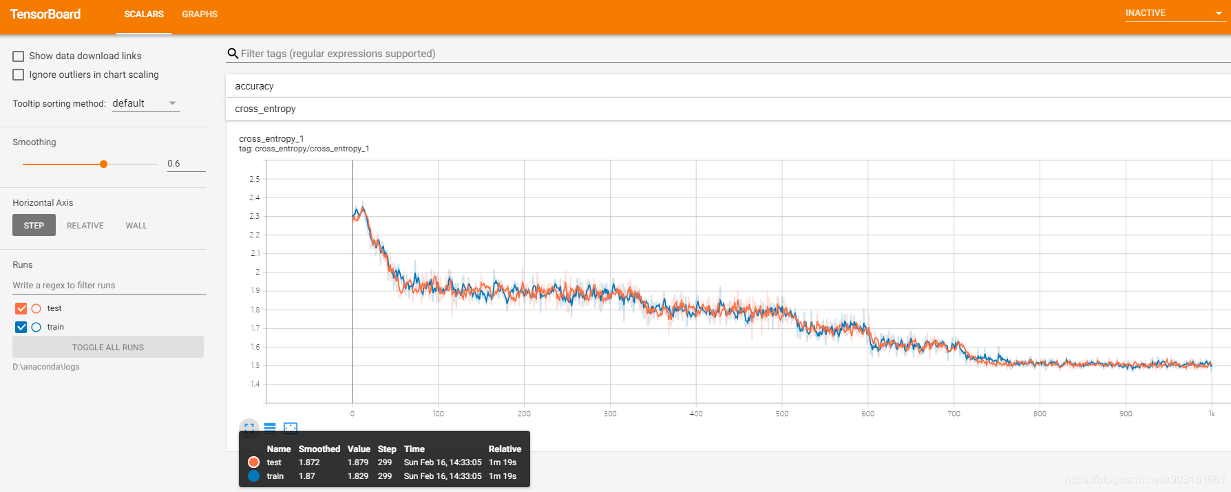
2.2.1.2 cross_entropy(交叉熵代价函数)

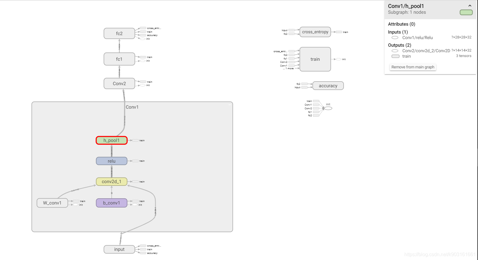
2.2.2 graphs

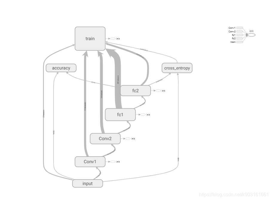
也可以单把网络拿出来(忽略我打开的这个第一卷积层)