Tensorflow学习-MNIST数据集

Tensorflow学习-MNIST数据集

Softmax

①数据集导入，keras自带的下载或者从某盘提取点击获取数据集，提取码：45yf

#导入数据集
from keras.datasets import mnist
(x_train,y_train),(x_test,y_test)=mnist.load_data('E:/TensorFlow_mnist/MNIST_data/mnist.npz')

print(x_train.shape,type(x_train))  #60000张28*28的图片
print(y_train.shape,type(y_train))  #60000个标签

②图像和数据类型的转化

#将图像28*28的转换成784
X_train = x_train.reshape(60000,784)
X_test = x_test.reshape(10000,784)
print(X_train.shape,type(X_train))
print(X_test.shape,type(X_test))


#将数据转换为float32
X_train=X_train.astype('float32')
X_test=X_test.astype('float32')
#数据归一化
X_train/=255
X_test/=255

③统计训练数据集中各标签的数量并可视化展示

#统计训练数据中的各标签数量
import numpy as np
import matplotlib.pyplot as plt

label,count=np.unique(y_train,return_counts=True)
print(label,count)
#lable的可视化输出
fig = plt.figure()
plt.bar(label,count,width=0.7,align='center')
plt.title("Label Distribution")
plt.xlabel("Label")
plt.ylabel("Count")
plt.xticks(label)
plt.ylim(0,7500)
for a,b in zip(label,count):
    plt.text(a,b,'%d' %b,ha='center',va='bottom',fontsize=10)
    
plt.show()

输出结果：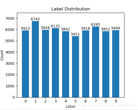

④标签编码
one-hot编码的实现

rom keras.utils import  np_utils

n_classes=10
print("Shape before one-hot encoding: ",y_train.shape)
Y_train=np.utils.to_categorical(y_train,n_classes)
print("Shape after one-hot encoding: ",Y_train.shape)
Y_test = np_utils.to_categorical(y_test,n_classes)

print(y_train[0])
print(Y_train[0])

可以看看输出为：

5 #one-hot之前的标签
[0. 0. 0. 0. 0. 1. 0. 0. 0. 0.]  #one-hot之后的标签

⑤定义神经网络
使用Keras sequential model定义神经网络

from keras.utils import  np_utils

n_classes=10
print("Shape before one-hot encoding: ",y_train.shape)
Y_train=np_utils.to_categorical(y_train,n_classes)
print("Shape after one-hot encoding: ",Y_train.shape)
Y_test = np_utils.to_categorical(y_test,n_classes)

# print(y_train[0])
# print(Y_train[0])

from keras.models import Sequential
from keras.layers.core import Dense,Activation

model = Sequential()
model.add(Dense(512,input_shape=(784,)))#全连接网络，512个神经元。输入784长度的向量对应输入的28*28
model.add(Activation('relu'))#激活函数选择relu

model.add(Dense(512))#全连接网络，512个神经元。输入的是上一层输出的数据
model.add(Activation('relu'))#激活函数为relu

model.add(Dense(10))
model.add(Activation('softmax'))

编译模型

model.compile(loss='categorical_crossentropy',metrics=['accuracy'],optimizer='adam')
#这一步之后得到了完整的数据流图

训练模型，并将指标保存到history中

history = model.fit(X_train,
                    Y_train,
                    batch_size=128,#每次128张图
                    epochs=5,#一共训练5次60000张图，总30W图
                    verbose=2,
                    validation_data=(X_test,Y_test))

结果显示：

Epoch 1/5
 - 7s - loss: 0.2156 - acc: 0.9358 - val_loss: 0.1063 - val_acc: 0.9676
Epoch 2/5
 - 5s - loss: 0.0797 - acc: 0.9757 - val_loss: 0.0754 - val_acc: 0.9764
Epoch 3/5
 - 5s - loss: 0.0496 - acc: 0.9842 - val_loss: 0.0675 - val_acc: 0.9778
Epoch 4/5
 - 5s - loss: 0.0345 - acc: 0.9889 - val_loss: 0.0745 - val_acc: 0.9780
Epoch 5/5
 - 5s - loss: 0.0249 - acc: 0.9918 - val_loss: 0.0763 - val_acc: 0.9790

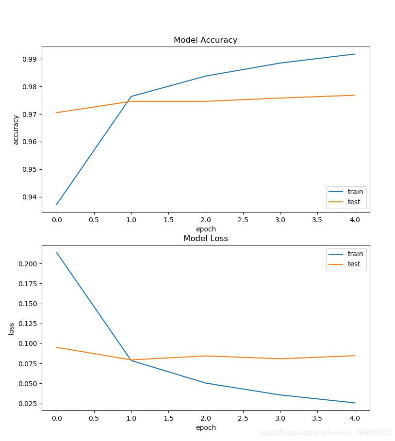
⑥指标可视化展示

fig = plt.figure()
plt.subplot(2,1,1)
plt.plot(history.history['acc'])
plt.plot(history.history['val_acc'])#测试集的准确率
plt.title('Model Accuracy')
plt.ylabel('accuracy')
plt.xlabel('epoch')
plt.legend(['train','test'],loc='lower right')

plt.subplot(2,1,2)
plt.plot(history.history['loss'])
plt.plot(history.history['val_loss'])
plt.title('Model Loss')
plt.ylabel('loss')
plt.xlabel('epoch')
plt.legend(['train','test'],loc='upper right')

plt.show()

图表展示：

⑦保存模型
keras将模型保存成HDF5文件格式

import os
import tensorflow.gfile as gfile

save_dir = "../TensorFlow_mnist/model"

if gfile.Exists(save_dir):
    gfile.DeleteRecursively(save_dir)
gfile.MakeDirs(save_dir)

model_name = 'keras_mnist.h5'
model_path=os.path.join(save_dir,model_name)
model.save(model_path)
print('Saved trained model at %s' %model_path)

保存为如下形式

⑧加载模型

from keras.models import load_model

mnist_modle = load_model(model_path)

loss_and_metrics=mnist_modle.evaluate(X_test,Y_test,verbose=2)

print("Test Loss:{}".format(loss_and_metrics[0]))
print("Test Accuracy:{}%".format(loss_and_metrics[1]*100))

predicted_classes = mnist_modle.predict_calsses(X_test)

correct_indices = np.nonzero(predicted_classes==y_test)[0]
incorrect_indices=np.nonzero(predicted_classes!=y_test)[0]
print("Classified correctly count: {}".format(len(correct_indices)))
print("Classified incorrectly count: {}".format(len(incorrect_indices)))