这篇博客主要是给大家分享下,Deep Learning 的入门级程序--Minst 的实现。主要程序是参考了《Tensorflow+实战Google深度学习框架》这本书中的源程。主要从如下三个方面来展开,首先是Minst数据集的简介,接着是具体的TensorFlow实现,最后是将训练后的模型具体的去应用,就是拿自己手写的单幅图去验证模型的实用性。
- Training set images: train-images-idx3-ubyte.gz (9.9 MB, 解压后 47 MB, 包含 60,000 个样本)
- Training set labels: train-labels-idx1-ubyte.gz (29 KB, 解压后 60 KB, 包含 60,000 个标签)
- Test set images: t10k-images-idx3-ubyte.gz (1.6 MB, 解压后 7.8 MB, 包含 10,000 个样本)
- Test set labels: t10k-labels-idx1-ubyte.gz (5KB, 解压后 10 KB, 包含 10,000 个标签)
这里着重强调两点,
1.Mnist 数据集里面的图片是以 一维的矩阵形式保存的,其长度为28*28=784。每一个值代表一个像素点的灰度值;2. 图片均是黑底白字,这和我们传统的白底黑字有很大不一样,这在第三部分,自己创建单幅图时要尤其要注意,如果用白底黑字的图片去识别,模型很容易识别错误。
二. Mnist 模型 具体代码实现
主要将代码分为三个模块,分别是 mnist_inference.py mnist_cnn_train.py mnist_def.py
其中
mnist_inference.py 主要是通过CNN 实现前向传播的功能 ;
mnist_cnn_train.py 实现了反向传播来更新参数;
mnist_def.py 主要是通过测试集来验证模型的准确率。具体原理不再赘述,详情可参考《Tensorflow+实战Google深度学习框架》
mnist_inference.py
import tensorflow as tf
# 定义神经网络相关的参数
INPUT_NODE=784
OUT_NODE=10


IMAGE_SIZE = 28
NUM_CHANNELS = 1
NUM_LABELS = 10

# 第一层卷积层的尺寸和深度
CONV1_DEEP = 32
CONV1_SIZE = 5
# 第二层卷积层的尺寸和深度
CONV2_DEEP = 64
CONV2_SIZE = 5
# 全连接层的节点个数
FC_SIZE = 512

# 定义神经网络的前向传播过程。
# 这里添加了一个新的参数train,用于区别训练过程和测试过程。
# 在这个程序中将用到dropout方法,dropout可以进一步提升模型可靠性并防止过拟合,dropout过程只在训练时使用。
def ff (input_tensor, train, regularizer):
    # 声明第一层神经网络的变量并完成前向传播过程。这个过程和6.3.1小节中介绍的一致。
    # 通过使用不同的命名空间来隔离不同层的变量,这可以让每一层中的变量命名只需要考虑在当前层的作用,而不需要担心重名的问题。
    # 和标准LeNet-5模型不大一样,这里定义卷积层的输入为28*28*1的原始MNIST图片像素。
    # 因为卷积层中使用了全0填充,所以输出为28*28*32的矩阵。
    with tf.variable_scope('layer1-conv1',reuse =tf.AUTO_REUSE):
        # 这里使用tf.get_variable或tf.Variable没有本质区别,因为在训练或是测试中没有在同一个程序中多次调用这个函数。
        # 如果在同一个程序中多次调用,在第一次调用之后需要将reuse参数置为True。
        conv1_weights = tf.get_variable(
            "weight", [CONV1_SIZE, CONV1_SIZE, NUM_CHANNELS, CONV1_DEEP],
            initializer = tf.truncated_normal_initializer(stddev=0.1)
        )
        conv1_biases = tf.get_variable("bias", [CONV1_DEEP], initializer=tf.constant_initializer(0.0))
        # 使用边长为5,深度为32的过滤器,过滤器移动的步长为1,且使用全0填充
        conv1 = tf.nn.conv2d(input_tensor, conv1_weights, strides=[1, 1, 1, 1], padding='SAME')
        relu1 = tf.nn.relu(tf.nn.bias_add(conv1, conv1_biases))

    # 实现第二层池化层的前向传播过程。
    # 这里选用最大池化层,池化层过滤器的边长为2,使用全0填充且移动的步长为2。
    # 这一层的输入是上一层的输出,也就是28*28*32的矩阵。输出为14*14*32的矩阵。
    with tf.name_scope('layer2-pool'):
        pool1 = tf.nn.max_pool(relu1, ksize=[1, 2, 2, 1], strides=[1, 2, 2, 1], padding='SAME')

    # 声明第三层卷积层的变量并实现前向传播过程。
    # 这一层的输入为14*14*32的矩阵,输出为14*14*64的矩阵。
    with tf.variable_scope('layer3-conv2',reuse =tf.AUTO_REUSE):
        conv2_weights = tf.get_variable(
            "weight", [CONV2_SIZE, CONV2_SIZE, CONV1_DEEP, CONV2_DEEP],
            initializer = tf.truncated_normal_initializer(stddev=0.1)
        )
        conv2_biases = tf.get_variable("bias", [CONV2_DEEP], initializer=tf.constant_initializer(0.0))
        # 使用边长为5,深度为64的过滤器,过滤器移动的步长为1,且使用全0填充
        conv2 = tf.nn.conv2d(pool1, conv2_weights, strides=[1, 1, 1, 1], padding='SAME')
        relu2 = tf.nn.relu(tf.nn.bias_add(conv2, conv2_biases))

    # 实现第四层池化层的前向传播过程。
    # 这一层和第二层的结构是一样的。这一层的输入为14*14*64的矩阵,输出为7*7*64的矩阵。
    with tf.name_scope('layer4-poo2'):
        pool2 = tf.nn.max_pool(relu2, ksize=[1, 2, 2, 1], strides=[1, 2, 2, 1], padding='SAME')

    # 将第四层池化层的输出转化为第五层全连接层的输入格式。
    # 第四层的输出为7*7*64的矩阵,然而第五层全连接层需要的输入格式为向量,所以在这里需要将这个7*7*64的矩阵拉直成一个向量。
    # pool2.get_shape函数可以得到第四层输出矩阵的维度而不需要手工计算。
    # 注意因为每一层神经网络的输入输出都为一个batch的矩阵,所以这里得到的维度也包含了一个batch中数据的个数。
    pool_shape = pool2.get_shape().as_list()
    # 计算将矩阵拉直成向量之后的长度,这个长度就是矩阵长度及深度的乘积。
    # 注意这里pool_shape[0]为一个batch中样本的个数。
    nodes = pool_shape[1] * pool_shape[2] * pool_shape[3]
    # 通过tf.reshape函数将第四层的输出变成一个batch的向量。
    reshaped = tf.reshape(pool2, [pool_shape[0], nodes])

    # 声明第五层全连接层的变量并实现前向传播过程。
    # 这一层的输入是拉直之后的一组向量,向量长度为7*7*64=3136,输出是一组长度为512的向量。
    # 这一层和之前在第5章中介绍的基本一致,唯一的区别是引入了dropout的概念。
    # dropout在训练时会随机将部分节点的输出改为0。
    # dropout可以避免过拟合问题,从而使得模型在测试数据上的效果更好。
    # dropout一般只在全连接层而不是卷积层或者池化层使用。
    with tf.variable_scope('layer5-fc1',reuse =tf.AUTO_REUSE):
        fc1_weights = tf.get_variable("weight", [nodes, FC_SIZE],
                                      initializer = tf.truncated_normal_initializer(stddev = 0.1))
        # 只有全连接层的权重需要加入正则化
        if regularizer != None:
            tf.add_to_collection('losses', regularizer(fc1_weights))
        fc1_biases = tf.get_variable('bias', [FC_SIZE], initializer = tf.constant_initializer(0.1))
        fc1 = tf.nn.relu(tf.matmul(reshaped, fc1_weights)+fc1_biases)
        if (train):
            fc1 = tf.nn.dropout(fc1, 0.5)

    # 声明第六层全连接层的变量并实现前向传播过程。
    # 这一层的输入是一组长度为512的向量,输出是一组长度为10的向量。
    # 这一层的输出通过Softmax之后就得到了最后的分类结果。
    with tf.variable_scope('layer6-fc2',reuse =tf.AUTO_REUSE):
        fc2_weights = tf.get_variable("weight", [FC_SIZE, NUM_LABELS],
                                      initializer = tf.truncated_normal_initializer(stddev = 0.1))
        if (regularizer != None):
            tf.add_to_collection('losses', regularizer(fc2_weights))
        fc2_biases = tf.get_variable('bias', [NUM_LABELS], initializer = tf.constant_initializer(0.1))
        logit = tf.matmul(fc1, fc2_weights) + fc2_biases

    # 返回第六层的输出
    return logit
mnist_cnn_train.py
import os
import numpy as np

import tensorflow as tf
from tensorflow.examples.tutorials.mnist import input_data

# 加载mnist_inference.py中定义的常量和前向传播的函数
import mnist_inference

# 配置神经网络的参数
BATCH_SIZE = 100
LEARNING_RATE_BASE = 0.01
LEARNING_RATE_DECAY = 0.99
REGULARAZTION_RATE = 0.0001
TRAINING_STEPS = 30000
MOVING_AVERAGE_DECAY = 0.99
# 模型保存的路径和文件名
MODEL_SAVE_PATH = "E:\TensorFlow\Project_TF\mnist_lenet_5\log"
MODEL_NAME ="model_minist.ckpt"

def train(mnist):
    # 定义输入输出placeholder
    # 调整输入数据placeholder的格式,输入为一个四维矩阵
    x = tf.placeholder(tf.float32, [
        BATCH_SIZE,                             # 第一维表示一个batch中样例的个数
        mnist_inference.IMAGE_SIZE,             # 第二维和第三维表示图片的尺寸
        mnist_inference.IMAGE_SIZE,
        mnist_inference.NUM_CHANNELS],          # 第四维表示图片的深度,对于RBG格式的图片,深度为5
                       name='x-input')
    y_ = tf.placeholder(tf.float32, [None, mnist_inference.OUT_NODE], name='y-input')
    regularizer = tf.contrib.layers.l2_regularizer(REGULARAZTION_RATE)
    # 直接使用mnist_inference.py中定义的前向传播过程
    y = mnist_inference.ff(x, True, regularizer)
    global_step = tf.Variable(0, trainable=False)

    #定义损失函数、学习率、滑动平均操作以及训练过程
    variable_averages = tf.train.ExponentialMovingAverage(MOVING_AVERAGE_DECAY, global_step)
    variable_averages_op = variable_averages.apply(tf.trainable_variables())
    cross_entropy = tf.nn.sparse_softmax_cross_entropy_with_logits(logits=y, labels=tf.argmax(y_, 1))
    cross_entropy_mean = tf.reduce_mean(cross_entropy)
    loss = cross_entropy_mean + tf.add_n(tf.get_collection('losses'))
    learning_rate = tf.train.exponential_decay(LEARNING_RATE_BASE, global_step, mnist.train.num_examples/BATCH_SIZE, LEARNING_RATE_DECAY)
    train_step = tf.train.GradientDescentOptimizer(learning_rate).minimize(loss, global_step=global_step)
    with tf.control_dependencies([train_step, variable_averages_op]):
        train_op = tf.no_op(name='train')

    # 初始化Tensorflow持久化类
    saver = tf.train.Saver()
    with tf.Session() as sess:
        tf.global_variables_initializer().run()
        # 验证和测试的过程将会有一个独立的程序来完成
        for i in range(TRAINING_STEPS):
            xs, ys = mnist.train.next_batch(BATCH_SIZE)
            #类似地将输入的训练数据格式调整为一个四维矩阵,并将这个调整后的数据传入sess.run过程
            reshaped_xs = np.reshape(xs, (BATCH_SIZE, mnist_inference.IMAGE_SIZE, mnist_inference.IMAGE_SIZE, mnist_inference.NUM_CHANNELS))
            _, loss_value, step = sess.run([train_op, loss, global_step], feed_dict={x: reshaped_xs, y_: ys})
            #每1000轮保存一次模型。
            if (i%1000) == 0:
                # 输出当前的训练情况。这里只输出了模型在当前训练batch上的损失函数大小。通过损失函数的大小可以大概了解训练的情况。
                # 在验证数据集上的正确率信息会有一个单独的程序来生成。
                print("After %d training step(s), loss on training batch is %f." % (step, loss_value))
                # 保存当前的模型。注意这里隔出了global_step参数,这样可以让每个被保存模型的文件名末尾加上训练的轮数,比如“model.ckpt-1000”表示训练1000轮后得到的模型
                saver.save(sess, os.path.join(MODEL_SAVE_PATH, MODEL_NAME), global_step=global_step)


def main(argv=None):
    mnist = input_data.read_data_sets("E:\TensorFlow\Project_TF\mnist_lenet_5\data", one_hot=True)
    train(mnist)


if (__name__ == '__main__'):  #如果是直接运行该该程序,则进入main函数,如果是调用该模块,则不运行main函数
    tf.app.run()
mnist_def.py
import numpy as np
import tensorflow as tf
from tensorflow.examples.tutorials.mnist import input_data

# 加载mnist_inference.py 和 mnist_train.py中定义的常量和函数
import mnist_inference
import mnist_train_cnn

# 每10秒加载一次最新的模型, 并在测试数据上测试最新模型的正确率


def evaluate (mnist):
    with tf.Graph().as_default() as g:
        # 定义输入输出的格式
        x= tf.placeholder(tf.float32, shape=(mnist.validation.num_examples,
                                          mnist_inference.IMAGE_SIZE,
                                          mnist_inference.IMAGE_SIZE,
                                          mnist_inference.NUM_CHANNELS), name='x-input')
        y_ = tf.placeholder(tf.float32, shape=(None, mnist_inference.OUT_NODE), name='y-input')

        validate_feed = {x: np.reshape(mnist.validation.images, (-1, mnist_inference.IMAGE_SIZE, mnist_inference.IMAGE_SIZE, mnist_inference.NUM_CHANNELS)),
                         y_: mnist.validation.labels}
        # 直接通过调用封装好的函数来计算前向传播的结果。
        # 因为测试时不关注正则损失的值,所以这里用于计算正则化损失的函数被设置为None。
        y = mnist_inference.ff(x, False, None)

        # 使用前向传播的结果计算正确率。
        # 如果需要对未知的样例进行分类,那么使用tf.argmax(y, 1)就可以得到输入样例的预测类别了。
        correct_prediction = tf.equal(tf.argmax(y, 1), tf.argmax(y_, 1))
        accuracy = tf.reduce_mean(tf.cast(correct_prediction, tf.float32))

        # 通过变量重命名的方式来加载模型,这样在前向传播的过程中就不需要调用求滑动平均的函数来获取平局值了。
        # 这样就可以完全共用mnist_inference.py中定义的前向传播过程
        variable_averages = tf.train.ExponentialMovingAverage(mnist_train_cnn.MOVING_AVERAGE_DECAY)
        variable_to_restore = variable_averages.variables_to_restore()
        saver = tf.train.Saver(variable_to_restore)
        with tf.Session() as sess:
                # tf.train.get_checkpoint_state函数会通过checkpoint文件自动找到目录中最新模型的文件名
                ckpt = tf.train.get_checkpoint_state(mnist_train_cnn.MODEL_SAVE_PATH)
                if ckpt and ckpt.model_checkpoint_path:
                    # 加载模型
                    saver.restore(sess, ckpt.model_checkpoint_path)
                    # 通过文件名得到模型保存时迭代的轮数
                    global_step = ckpt.model_checkpoint_path.split('/')[-1].split('-')[-1]
                    accuracy_score = sess.run(accuracy, feed_dict = validate_feed)
                    print("After %s training step(s), validation accuracy = %f" % (global_step, accuracy_score))
                else:
                    print("No checkpoint file found")
                    return

def main(argv=None):
    mnist = input_data.read_data_sets("E:\TensorFlow\Project_TF\mnist_lenet_5\data", one_hot=True)
    evaluate(mnist)


if __name__ == '__main__':
    tf.app.run()
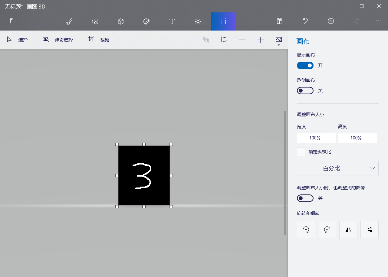
三. 模型的实际应用
通过win10自带的3D绘图功能,可以自己手动书写数字,最好是将画布调成黑色的,然后再用白色的像素笔书写
。在这里还要强调一点,最后保存时需要将图片裁剪的小一些,因为训练时图片的数据都是28*28的,如果输入图片太大话,会因为图片缩小比例太大,造成识别率降低。

最终缩小后的图片
mnist_recognize_one.py
import tensorflow as tf
import numpy as np
import mnist_inference
import mnist_train_cnn
import cv2
import matplotlib.pyplot as plt
'''如果自己手写的图片是白底黑字的话,可以通过该函数将图片灰度值反转'''
#def reversePic(src):
# # 图像反转
# for i in range(src.shape[0]):
# for j in range(src.shape[1]):
# src[i,j] = 255 - src[i,j]
# return src
def main():
#识别一张图片
sess = tf.InteractiveSession() #定义会话
test_dir="E:\\TensorFlow\\Project_TF\\mnist_lenet_5\\data\\test\\3.jpg"
x = tf.placeholder(tf.float32, (1, #因为要识别的图片只有一张,所以对应的batch_size为1
mnist_inference.IMAGE_SIZE, # 第二维和第三维表示图片的尺寸
mnist_inference.IMAGE_SIZE,
mnist_inference.NUM_CHANNELS), # 第四维表示图片的深度,对于RBG格式的图片,深度为5
name='x-input')
y=mnist_inference.ff(x,False,None)
y_result=tf.nn.softmax(y) #输出层,使用softmax进行多分类
im = cv2.imread( test_dir,cv2.IMREAD_GRAYSCALE)
# im =reversePic(im) #图像灰度值反转,如果有需要的话
plt.matshow(im)
im = cv2.resize(im,(28,28),interpolation=cv2.INTER_CUBIC) #图片预处理,统一成28*28
x_img = np.reshape(im , (1,28,28,1)) #将图片变成四维的
'''重新加载模型保存的参数'''
variable_averages=tf.train.ExponentialMovingAverage(mnist_train_cnn.MOVING_AVERAGE_DECAY)
variable_to_restore=variable_averages.variables_to_restore()
saver=tf.train.Saver(variable_to_restore)
ckpt=tf.train.get_checkpoint_state(mnist_train_cnn.MODEL_SAVE_PATH)
saver.restore(sess,ckpt.model_checkpoint_path)
output = sess.run( y_result , feed_dict = {x:x_img})
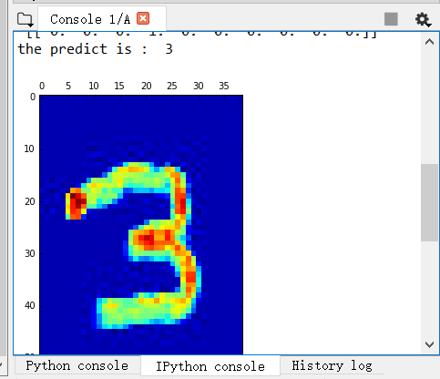
print ('the y_con : ', '\n',output ) #输出对应每个数的概率
print ('the predict is : ', np.argmax(output)) #输出最大概率所对应的标签
#关闭会话
sess.close()
if (__name__ == '__main__'):
main()
最后识别后的结果如下图所示
新手开博,刚入坑机器学习半年有余,如果有哪里写的不对的地方,还请各位大牛予以指出,定不胜感激。还望共同进步!
