预设:导入相关包,设置相关数据(这里借鉴了这位博主的笔记,很详实Google TensorFlow课程 编程笔记(2)———使用TensorFlow的基本步骤)
from __future__ import print_function
from IPython import display    #display模块可以决定显示的内容以何种格式显示
from matplotlib import cm    # matplotlib为python的2D绘图库# cm为颜色映射表
from matplotlib import gridspec    # 使用 GridSpec 自定义子图位置
from matplotlib import pyplot as plt    # pyplot提供了和matlab类似的绘图API,方便用户快速绘制2D图表
import numpy as np    # numpy为python的科学计算包,提供了许多高级的数值编程工具
import pandas as pd    # pandas是基于numpy的数据分析包,是为了解决数据分析任务而创建的
from sklearn import metrics    # sklearn(scikit-_learn_)是一个机器学习算法库,包含了许多种机器学习的方式
# * Classification 分类# * Regression 回归
# * Clustering 非监督分类# * Dimensionality reduction 数据降维
# * Model Selection 模型选择# * Preprocessing 数据预处理
# metrics:度量(字面意思),它提供了很多模块可以为第三方库或者应用提供辅助统计信息
import tensorflow as tf    # tensorflow是谷歌的机器学习框架
from tensorflow.python.data import Dataset    # Dataset无比强大得数据集
tf.logging.set_verbosity(tf.logging.ERROR)
pd.options.display.max_rows = 10    # 为了观察数据方便,最多只显示10行数据
pd.options.display.float_format = '{:.1f}'.format
california_housing_dataframe = pd.read_csv("https://storage.googleapis.com/mledu-datasets/california_housing_train.csv", sep=",")
 #加载数据集
california_housing_dataframe = california_housing_dataframe.reindex(
    np.random.permutation(california_housing_dataframe.index))
california_housing_dataframe["median_house_value"] /= 1000.0
california_housing_dataframe    #对数据进行预处理将median_house_value调整为以千为单位。
california_housing_dataframe.describe()    #检查数据
模型构建
下面开始第一个模型的构建
第 1 步:定义特征并配置特征列
为了将我们的训练数据导入 TensorFlow,我们需要指定每个特征包含的数据类型。在本练习及今后的练习中,我们主要会使用以下两类数据:
分类数据: 一种文字数据。在本练习中,我们的住房数据集不包含任何分类特征,但您可能会看到的示例包括家居风格以及房地产广告词。
数值数据: 一种数字(整数或浮点数)数据以及您希望视为数字的数据。有时您可能会希望将数值数据(例如邮政编码)视为分类数据(我们将在稍后的部分对此进行详细说明)。
在 TensorFlow 中,我们使用一种称为“特征列”的结构来表示特征的数据类型。特征列仅存储对特征数据的描述;不包含特征数据本身。
一开始,我们只使用一个数值输入特征 total_rooms。以下代码会从 california_housing_dataframe 中提取 total_rooms 数据,并使用 numeric_column 定义特征列,这样会将其数据指定为数值:
特征列的详细知识转到该链接Tensorflow特征列
# 这里使用两个中括号的原因:
# california_housing_dataframe[['total_rooms']]内层中括号获取total_rooms对应的Series,而外层括号以该Series建立一个DataSet,其中只含这一列数据Series,这样可以表示仅有这一列被保留下来使用、
#my_feature是一个DataSet
my_feature = california_housing_dataframe[["total_rooms"]]# Define the input feature: total_rooms.
# 获取特征列:特征列是将原始数据转换成机器能识别处理的一种格式。特征列在输入数据(由 input_fn 返回)与模型之间架起了桥梁,通过处理特征列可以映射到特征上,特征列是存储分类信息的集合,具体使用时需将特征集合和特征列结合起来。
feature_columns = [tf.feature_column.numeric_column("total_rooms")]# Configure a numeric feature column for total_rooms.
第 2 步:定义目标
接下来,我们将定义目标,也就是 median_house_value。同样,我们可以从 california_housing_dataframe 中提取它:
# Define the label.
#这里控制的返回是Series
targets = california_housing_dataframe["median_house_value"]
第 3 步:配置 LinearRegressor
接下来,我们将使用 LinearRegressor 配置线性回归模型,并使用 GradientDescentOptimizer(它会实现小批量随机梯度下降法 (SGD))训练该模型。learning_rate 参数可控制梯度步长的大小。
注意:为了安全起见,我们还会通过 clip_gradients_by_norm 将梯度裁剪应用到我们的优化器。梯度裁剪可确保梯度大小在训练期间不会变得过大,梯度过大会导致梯度下降法失败。
# Use gradient descent as the optimizer for training the model.
# 实现线性回归模型,设置学习率,在这里使用的是SGD
my_optimizer = tf.train.GradientDescentOptimizer(learning_rate=0.0000001)
# 这里的clip_by_norm是指对梯度进行裁剪并应用到优化器中,通过控制梯度的最大范式,防止梯度爆炸,梯度过大会导致梯度下降法失败。语法:API.clip_gradients_by_norm(优化器,梯度上限)
my_optimizer = tf.contrib.estimator.clip_gradients_by_norm(my_optimizer, 5.0)
# my_optimizer = tf.estimator.clip_gradients_by_norm(my_optimizer, 5.0)

# Configure the linear regression model with our feature columns and optimizer.
# Set a learning rate of 0.0000001 for Gradient Descent.
# 用特征列和梯度下降模型定义线性回归模型
linear_regressor = tf.estimator.LinearRegressor(
    feature_columns=feature_columns,
    optimizer=my_optimizer
)
第 4 步:定义输入函数
要将加利福尼亚州住房数据导入 LinearRegressor,我们需要定义一个输入函数,让它告诉 TensorFlow 如何对数据进行预处理,以及在模型训练期间如何批处理、随机处理和重复数据。
首先,我们将 Pandas 特征数据转换成 NumPy 数组字典。然后,我们可以使用 TensorFlow Dataset API 根据我们的数据构建 Dataset 对象,并将数据拆分成大小为 batch_size 的多批数据,以按照指定周期数 (num_epochs) 进行重复。
注意:如果将默认值 num_epochs=None 传递到 repeat(),输入数据会无限期重复。
然后,如果 shuffle 设置为 True,则我们会对数据进行随机处理,以便数据在训练期间以随机方式传递到模型。buffer_size 参数会指定 shuffle 将从中随机抽样的数据集的大小。
最后,输入函数会为该数据集构建一个迭代器,并向 LinearRegressor 返回下一批数据。
def my_input_fn(features, targets, batch_size=1, shuffle=True, num_epochs=None):
    """Trains a linear regression model of one feature.

    Args:
      features: pandas DataFrame of features
      targets: pandas DataFrame of targets
      batch_size: Size of batches to be passed to the model
      shuffle: True or False. Whether to shuffle the data.
      num_epochs: Number of epochs for which data should be repeated. None = repeat indefinitely
    Returns:
      Tuple of (features, labels) for next data batch
    """

    # Convert pandas data into a dict of np arrays.

	# dict(features).items():将输入的特征值转换为dictinary(python的一种数据类型),通过for语句遍历,得到其所有的一一对应的值(key:value)
    features = {key:np.array(value) for key,value in dict(features).items()}

    # Construct a dataset, and configure batching/repeating.
	# Dataset.from_tensor_slices((features,targets))将输入的两个参数拼接组合起来(feature1,target1),(feature2,target2)
    ds = Dataset.from_tensor_slices((features,targets)) # warning: 2GB limit
    # 将ds数据集按照batch_size大小组合成一个batch并以num_epochs的周期重复读取下去
    ds = ds.batch(batch_size).repeat(num_epochs)

    # Shuffle the data, if specified.
    # 现在ds中的数据集已经时按照batchsize组合成得一个一个batch,存放在队列中,并且重复了n次,这样子的话,不断重复,后面数据没有意义,所以将其随机打乱,每次取出butter_size的大小
 if shuffle:
      ds = ds.shuffle(buffer_size=10000)

    # Return the next batch of data.
    # make_one_shot_iterator().get_next():用迭代器迭代并在执行过程中返回所有的结果
    features, labels = ds.make_one_shot_iterator().get_next()
    return features, labels
第 5 步:训练模型
现在,我们可以在 linear_regressor 上调用 train() 来训练模型。我们会将 my_input_fn 封装在 lambda 中,以便可以将 my_feature 和 target 作为参数传入(有关详情,请参阅 TensorFlow 输入函数教程),首先,我们会训练 100 步。
_ = linear_regressor.train(
    input_fn = lambda:my_input_fn(my_feature, targets),
    steps=100
)
第 6 步:评估模型
我们基于该训练数据做一次预测,看看我们的模型在训练期间与这些数据的拟合情况。
**注意:训练误差可以衡量您的模型与训练数据的拟合情况,但并不能衡量模型泛化到新数据的效果。**在后面的练习中,您将探索如何拆分数据以评估模型的泛化能力。
# Create an input function for predictions.
# Note: Since we're making just one prediction for each example, we don't
# need to repeat or shuffle the data here.
# 下面三步是在已经训练完10000步之后获取得到的结果
prediction_input_fn =lambda: my_input_fn(my_feature, targets, num_epochs=1, shuffle=False)

# Call predict() on the linear_regressor to make predictions.
predictions = linear_regressor.predict(input_fn=prediction_input_fn)

# Format predictions as a NumPy array, so we can calculate error metrics.
predictions = np.array([item['predictions'][0] for item in predictions])
# 使用均方损失公式计算均方误差
# Print Mean Squared Error and Root Mean Squared Error.
mean_squared_error = metrics.mean_squared_error(predictions, targets)
# 对均方误差开根获取均方根误差
root_mean_squared_error = math.sqrt(mean_squared_error)
# 输出比较
print("Mean Squared Error (on training data): %0.3f" % mean_squared_error)
print("Root Mean Squared Error (on training data): %0.3f" % root_mean_squared_error)
结果:

误差分析
构建完成之后,我们来找一种适合且有效的误差分析方法
由于均方误差 (MSE) 很难解读,因此我们经常查看的是均方根误差 (RMSE)。RMSE 的一个很好的特性是,它可以在与原目标相同的规模下解读。
我们来比较一下 RMSE 与目标最大值和最小值的差值:
min_house_value = california_housing_dataframe["median_house_value"].min()
max_house_value = california_housing_dataframe["median_house_value"].max()
min_max_difference = max_house_value - min_house_value

print("Min. Median House Value: %0.3f" % min_house_value)
print("Max. Median House Value: %0.3f" % max_house_value)
print("Difference between Min. and Max.: %0.3f" % min_max_difference)
print("Root Mean Squared Error: %0.3f" % root_mean_squared_error)
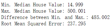
我们的误差跨越目标值的近一半范围,可以进一步缩小误差吗?
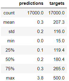
首先,我们可以了解一下根据总体摘要统计信息,预测和目标的符合情况。
calibration_data = pd.DataFrame()
calibration_data["predictions"] = pd.Series(predictions)
calibration_data["targets"] = pd.Series(targets)
calibration_data.describe()
我们还可以将数据和学到的线可视化。我们已经知道,单个特征的线性回归可绘制成一条将输入 x 映射到输出 y 的线。
首先,我们将获得均匀分布的随机数据样本,以便绘制可辨的散点图。然后,我们根据模型的偏差项和特征权重绘制学到的线,并绘制散点图。该线会以红色显示。
#获取随机数据模型
sample = california_housing_dataframe.sample(n=300)
# Get the min and max total_rooms values.
x_0 = sample["total_rooms"].min()
x_1 = sample["total_rooms"].max()

# Retrieve the final weight and bias generated during training.
# 从目前的训练模型中取出训练得到的weight(权重)和bias(偏差)
weight = linear_regressor.get_variable_value('linear/linear_model/total_rooms/weights')[0]
bias = linear_regressor.get_variable_value('linear/linear_model/bias_weights')

# Get the predicted median_house_values for the min and max
# 使用目前训练得到的权值去预测出x_0和x_1对应的y_0和y_1,这样可以得到预测的两个点的坐标,从而获得直线
total_rooms values.
y_0 = weight * x_0 + bias
y_1 = weight * x_1 + bias

# Plot our regression line from (x_0, y_0) to (x_1, y_1).
# 画图
plt.plot([x_0, x_1], [y_0, y_1], c='r')
# Label the graph axes.
plt.ylabel("median_house_value")
plt.xlabel("total_rooms")
# Plot a scatter plot from our data sample.
plt.scatter(sample["total_rooms"], sample["median_house_value"])
# Display graph.
plt.show()

调整超参数
为方便起见,已将上述所有代码放入一个函数中。可以使用不同的参数调用该函数,以了解相应效果。
我们会在 10 个等分的时间段内使用此函数,以便观察模型在每个时间段的改善情况。
对于每个时间段,我们都会计算训练损失并绘制相应图表。这可以帮助您判断模型收敛的时间,或者模型是否需要更多迭代。
此外,我们还会绘制模型随着时间的推移学习的特征权重和偏差项值的曲线图。您还可以通过这种方式查看模型的收敛效果。
def train_model(learning_rate, steps, batch_size, input_feature="total_rooms"):
"""Trains a linear regression model of one feature.
Args:
learning_rate: A `float`, the learning rate.
steps: A non-zero `int`, the total number of training steps. A training step
consists of a forward and backward pass using a single batch.
batch_size: A non-zero `int`, the batch size.
input_feature: A `string` specifying a column from `california_housing_dataframe`
to use as input feature.
"""
# 将步长分十份,用于每训练十分之一的步长就输出一次结果
periods = 10
steps_per_period = steps / periods
# 数据准备
my_feature = input_feature
# 获取特征集合
my_feature_data = california_housing_dataframe[[my_feature]]
# 获取目标集合
my_label = "median_house_value"
targets = california_housing_dataframe[my_label]
# 获取特征列
# Create feature columns.
feature_columns = [tf.feature_column.numeric_column(my_feature)]
# 进行输入量的训练
# Create input functions.
training_input_fn = lambda:my_input_fn(my_feature_data, targets, batch_size=batch_size)
prediction_input_fn = lambda: my_input_fn(my_feature_data, targets, num_epochs=1, shuffle=False)
# 设置模型
# Create a linear regressor object.
my_optimizer = tf.train.GradientDescentOptimizer(learning_rate=learning_rate)
my_optimizer = tf.contrib.estimator.clip_gradients_by_norm(my_optimizer, 5.0)
linear_regressor = tf.estimator.LinearRegressor(
feature_columns=feature_columns,
optimizer=my_optimizer
)
# Set up to plot the state of our model's line each period.
# 设置绘画参数
# 新建绘画窗口,自定义画布的大小为15*6
plt.figure(figsize=(15, 6))
# 设置画布划分以及图像在画布上输出的位置1行2列,绘制在第1个位置
plt.subplot(1, 2, 1)
plt.title("Learned Line by Period")
plt.ylabel(my_label)
plt.xlabel(my_feature)
sample = california_housing_dataframe.sample(n=300)
# 绘制散点图
plt.scatter(sample[my_feature], sample[my_label])
# np.linspace(-1, 1, periods):用于输出等差数列,起始-1,结尾1,periods=10,10等分(不写的话默认50等分)
# cm.coolwarm(x):设置颜色,用于十条线显示不同颜色
colors = [cm.coolwarm(x) for x in np.linspace(-1, 1, periods)]
# Train the model, but do so inside a loop so that we can periodically assess
# loss metrics.
print("Training model...")
print("RMSE (on training data):")
# 变量:均方根误差
root_mean_squared_errors = []
# 从0到10进行绘制,获得不同时间段的训练情况
for period in range (0, periods):
# Train the model, starting from the prior state.
linear_regressor.train(
input_fn=training_input_fn,
steps=steps_per_period
)
# Take a break and compute predictions.
predictions = linear_regressor.predict(input_fn=prediction_input_fn)
predictions = np.array([item['predictions'][0] for item in predictions])
# Compute loss.
root_mean_squared_error = math.sqrt(
metrics.mean_squared_error(predictions, targets))
# Occasionally print the current loss.
print(" period %02d : %0.2f" % (period, root_mean_squared_error))
# Add the loss metrics from this period to our list.
root_mean_squared_errors.append(root_mean_squared_error)
# Finally, track the weights and biases over time.
# Apply some math to ensure that the data and line are plotted neatly.
y_extents = np.array([0, sample[my_label].max()])
weight = linear_regressor.get_variable_value('linear/linear_model/%s/weights' % input_feature)[0]
bias = linear_regressor.get_variable_value('linear/linear_model/bias_weights')
x_extents = (y_extents - bias) / weight
x_extents = np.maximum(np.minimum(x_extents,
sample[my_feature].max()),
sample[my_feature].min())
y_extents = weight * x_extents + bias
plt.plot(x_extents, y_extents, color=colors[period])
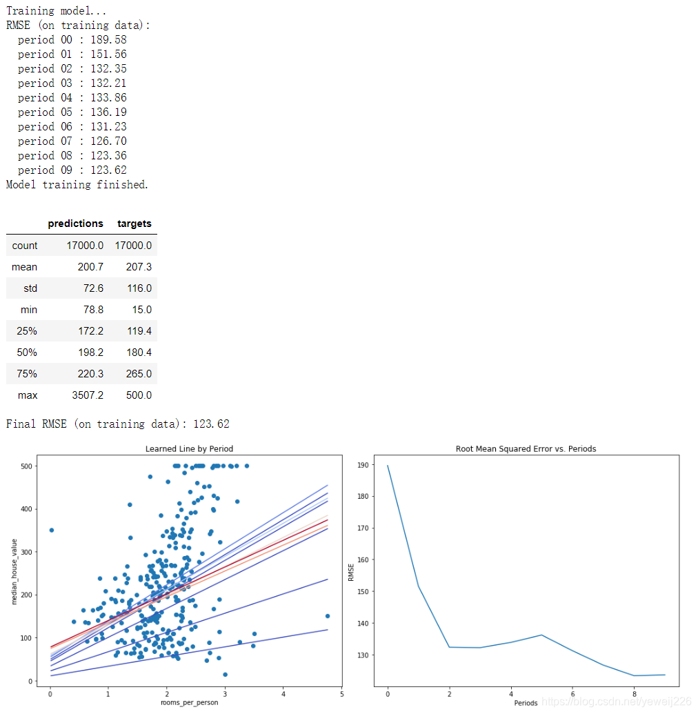
print("Model training finished.")
# 输出RMSE曲线图
# Output a graph of loss metrics over periods.
plt.subplot(1, 2, 2)
plt.ylabel('RMSE')
plt.xlabel('Periods')
plt.title("Root Mean Squared Error vs. Periods")
plt.tight_layout()
plt.plot(root_mean_squared_errors)
# 输出预测目标值的对比
# Output a table with calibration data.
calibration_data = pd.DataFrame()
calibration_data["predictions"] = pd.Series(predictions)
calibration_data["targets"] = pd.Series(targets)
display.display(calibration_data.describe())
print("Final RMSE (on training data): %0.2f" % root_mean_squared_error)
设置相关参数:
train_model(
    learning_rate=0.00001,
    steps=100,
    batch_size=1
)

任务 1:使 RMSE 不超过 180
解决办法:使用以下参数
train_model(
    learning_rate=0.0002,
    steps=500,
    batch_size=100
)

任务 2:尝试其他特征
使用 population 特征替换 total_rooms 特征,看看能否取得更好的效果。
train_model(
    learning_rate=0.00002,
    steps=1000,
    batch_size=5,
    input_feature="population"
)

任务 3:尝试合成特征
total_rooms 和 population 特征都会统计指定街区的相关总计数据。
但是,如果一个街区比另一个街区的人口更密集,会怎么样?我们可以创建一个合成特征(即 total_rooms 与 population 的比例)来探索街区人口密度与房屋价值中位数之间的关系。
california_housing_dataframe["rooms_per_person"] = pd.Series(
california_housing_dataframe["total_rooms"] / california_housing_dataframe["population"])

calibration_data = train_model(
    learning_rate=1,
    steps=50,
    batch_size=100,
    input_feature="rooms_per_person"
)
任务 4:识别离群值
我们可以通过创建预测值与目标值的散点图来可视化模型效果。理想情况下,这些值将位于一条完全相关的对角线上。
使用您在任务 1 中训练过的人均房间数模型,并使用 Pyplot 的 scatter() 创建预测值与目标值的散点图。
# YOUR CODE HERE
plt.figure(figsize=(15, 6))
plt.subplot(1, 2, 1)
plt.scatter(calibration_data["predictions"], calibration_data["targets"])

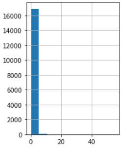
校准数据显示,大多数散点与一条线对齐。这条线几乎是垂直的,我们稍后再讲解。现在,我们重点关注偏离这条线的点。我们注意到这些点的数量相对较少。
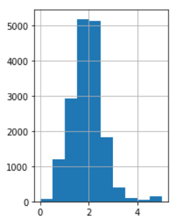
如果我们绘制 rooms_per_person 的直方图,则会发现我们的输入数据中有少量离群值:
plt.subplot(1, 2, 2)
_ = california_housing_dataframe["rooms_per_person"].hist()
任务 5:截取离群值
通过将 rooms_per_person 的离群值设置为相对合理的最小值或最大值来进一步改进模型拟合情况。
# YOUR CODE HERE
clipped_feature = california_housing_dataframe["rooms_per_person"].apply(lambda x:min(x,5))
plt.subplot(1,2,2)
_=clipped_feature.hist()
calibration_data = train_model(
    learning_rate=0.05,
    steps=500,
    batch_size=5,
    input_feature="rooms_per_person")

