首先引入一些比较重要的概念
**特征工程
概念:将原始数据转换为特征矢量。许多机器学习模型都必须将特征表示为实数向量,因为特征值必须与模型权重相乘。
特征工程分类:
1、映射数值:直接取值,不需要特殊编码
2、映射分类:需要特殊编码。分类特征具有一组离散的可能值。
如:
{‘Charleston Road’, ‘North Shoreline Boulevard’, ‘Shorebird Way’, ‘Rengstorff Avenue’}
由于模型不能将字符串与学习到的权重相乘,因此我们使用特征工程将字符串转换为数字值。
方法一:
要实现这一点,我们可以定义一个从特征值(我们将其称为可能值的词汇表)到整数的映射。世界上的每条街道并非都会出现在我们的数据集中,因此我们可以将所有其他街道分组为一个全部包罗的“其他”类别,称为 OOV(词汇表外)分桶。
如:
将 Charleston Road 映射到 0
将 North Shoreline Boulevard 映射到 1
将 Shorebird Way 映射到 2
将 Rengstorff Avenue 映射到 3
将所有其他街道 (OOV) 映射到 4
缺点:
①含一定顺序,不灵活
②若一项含多个值,该方法无法实现要求
方法二:
可以为模型中的每个分类特征创建一个二元向量来表示这些值,如下所述:
对于适用于样本的值,将相应向量元素设为 1。
将所有其他元素设为 0。
该向量的长度等于词汇表中的元素数。当只有一个值为 1 时,这种表示法称为独热编码;当有多个值为 1 时,这种表示法称为多热编码。

如图所示为街道 Shorebird Way 的独热编码。在此二元矢量中,代表 Shorebird Way 的元素的值为 1,而代表所有其他街道的元素的值为 0。
当然,假设数据集中有 100 万个不同的街道名称,您希望将其包含为 street_name 的值。如果直接创建一个包含 100 万个元素的二元向量,其中只有 1 或 2 个元素为 ture,则是一种非常低效的表示法,在处理这些向量时会占用大量的存储空间并耗费很长的计算时间。在这种情况下,一种常用的方法是使用稀疏表示法,其中仅存储非零值。 在稀疏表示法中,仍然为每个特征值学习独立的模型权重。
良好特征
在机器学习中我们更希望使用良好特征,那么良好特征的特点有:
①避免使用频率很少的离散特征值
②特征值最好有清晰明确的定义
③实际数据内不要掺入特殊值
如果用户没有输入 quality_rating,则数据集可能使用如下特殊值来表示不存在该值:quality_rating: -1
为解决特殊值的问题,需将该特征转换为两个特征:
一个特征只存储质量评分,不含特殊值。
一个特征存储布尔值,表示是否提供了 quality_rating。为该布尔值特征指定一个名称,例如 is_quality_rating_defined。
④考虑上游不稳定性:特征的定义不应随时间发生变化。
清理数据:将不可使用的样本消除
清查:
- 遗漏值。 例如,有人忘记为某个房屋的年龄输入值。
- 重复样本。 例如,服务器错误地将同一条记录上传了两次。
- 不良标签。例如,有人错误地将一颗橡树的图片标记为枫树。
- 不良特征值。 例如,有人输入了多余的位数,或者温度计被遗落在太阳底下。
除了检测各个不良样本之外,您还必须检测集合中的不良数据。直方图是一种用于可视化集合中数据的很好机制。此外,收集如下统计信息也会有所帮助:
- 最大值和最小值
- 均值和中间值
- 标准偏差
清理数据的基本方法:
1、缩放特征值:如果特征集包含多个特征,则缩放特征可以带来以下优势:
- 帮助梯度下降法更快速地收敛。
- 帮助避免“NaN 陷阱”。在这种陷阱中,模型中的一个数值变成 NaN(例如,当某个值在训练期间超出浮点精确率限制时),并且模型中的所有其他数值最终也会因数学运算而变成 NaN。
- 帮助模型为每个特征确定合适的权重。如果没有进行特征缩放,则模型会对范围较大的特征投入过多精力。
要缩放数字数据,一种显而易见的方法是将 [最小值,最大值] 以线性方式映射到较小的范围,例如 [-1,+1]。另一种热门的缩放策略是计算每个值的 Z 得分。Z 得分与距离均值的标准偏差数相关。换而言之: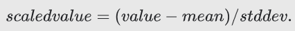
2、处理极端离群值:
①对每个值取对数,缩小极端
②将特征的最大值或最小值“限制”为某个任意值(比如 4.0)。将特征值限制到 4.0 并不意味着我们会忽略所有大于 4.0 的值。而是说,所有大于 4.0 的值都将变成 4.0。这就解释了 4.0 处的那个有趣的小峰值。
3、分箱:
下面的曲线图显示了加利福尼亚州不同纬度的房屋相对普及率。注意集群 - 洛杉矶大致在纬度 34 处,旧金山大致在纬度 38 处。

每个纬度的房屋数曲线图。曲线图极其不规则,在纬度 36 左右出现低谷,并在纬度 34 和 38 左右出现巨大峰值。
在数据集中,latitude 是一个浮点值。不过,在我们的模型中将 latitude 表示为浮点特征没有意义。这是因为纬度和房屋价值之间不存在线性关系。例如,纬度 35 处的房屋并不比纬度 34 处的房屋贵 35/34(或更便宜)。但是,纬度或许能很好地预测房屋价值。
为了将纬度变为一项实用的预测指标,我们对纬度“分箱”,如下图所示:

我们现在拥有 11 个不同的布尔值特征(LatitudeBin1、LatitudeBin2、…、LatitudeBin11),而不是一个浮点特征。拥有 11 个不同的特征有点不方便,因此我们将它们统一成一个 11 元素矢量。这样做之后,我们可以将纬度 37.4 表示为:
[0, 0, 0, 0, 0, 1, 0, 0, 0, 0, 0]
分箱之后,我们的模型现在可以为每个纬度学习完全不同的权重。
为了简单起见,我们在纬度样本中使用整数作为分箱边界。如果我们需要更精细的解决方案,我们可以每隔 1/10 个纬度拆分一次分箱边界。添加更多箱可让模型从纬度 37.4 处学习和维度 37.5 处不一样的行为,但前提是每 1/10 个纬度均有充足的样本可供学习。
另一种方法是按分位数分箱,这种方法可以确保每个桶内的样本数量是相等的。按分位数分箱完全无需担心离群值。
下面是编程练习:
基础包与函数的设置(若有问题可转到Google 机器学习编程笔记三——回归模型的验证查看相关代码)
from __future__ import print_function

import math

from IPython import display
from matplotlib import cm
from matplotlib import gridspec
from matplotlib import pyplot as plt
import numpy as np
import pandas as pd
from sklearn import metrics
import tensorflow as tf
from tensorflow.python.data import Dataset

tf.logging.set_verbosity(tf.logging.ERROR)
pd.options.display.max_rows = 10
pd.options.display.float_format = '{:.1f}'.format

california_housing_dataframe = pd.read_csv("https://download.mlcc.google.cn/mledu-datasets/california_housing_train.csv", sep=",")

california_housing_dataframe = california_housing_dataframe.reindex(
    np.random.permutation(california_housing_dataframe.index))
def preprocess_features(california_housing_dataframe):
  """Prepares input features from California housing data set.

  Args:
    california_housing_dataframe: A Pandas DataFrame expected to contain data
      from the California housing data set.
  Returns:
    A DataFrame that contains the features to be used for the model, including
    synthetic features.
  """
  selected_features = california_housing_dataframe[
    ["latitude",
     "longitude",
     "housing_median_age",
     "total_rooms",
     "total_bedrooms",
     "population",
     "households",
     "median_income"]]
  processed_features = selected_features.copy()
  # Create a synthetic feature.
  processed_features["rooms_per_person"] = (
    california_housing_dataframe["total_rooms"] /
    california_housing_dataframe["population"])
  return processed_features

def preprocess_targets(california_housing_dataframe):
  """Prepares target features (i.e., labels) from California housing data set.

  Args:
    california_housing_dataframe: A Pandas DataFrame expected to contain data
      from the California housing data set.
  Returns:
    A DataFrame that contains the target feature.
  """
  output_targets = pd.DataFrame()
  # Scale the target to be in units of thousands of dollars.
  output_targets["median_house_value"] = (
    california_housing_dataframe["median_house_value"] / 1000.0)
  return output_targets
# Choose the first 12000 (out of 17000) examples for training.
training_examples = preprocess_features(california_housing_dataframe.head(12000))
training_targets = preprocess_targets(california_housing_dataframe.head(12000))

# Choose the last 5000 (out of 17000) examples for validation.
validation_examples = preprocess_features(california_housing_dataframe.tail(5000))
validation_targets = preprocess_targets(california_housing_dataframe.tail(5000))

# Double-check that we've done the right thing.
print("Training examples summary:")
display.display(training_examples.describe())
print("Validation examples summary:")
display.display(validation_examples.describe())

print("Training targets summary:")
display.display(training_targets.describe())
print("Validation targets summary:")
display.display(validation_targets.describe())

使用之前的练习内容接着练习特征值的选取,如代码中有问题可见Google 机器学习编程笔记三——回归模型的验证查看相关代码注释
def construct_feature_columns(input_features):
  """Construct the TensorFlow Feature Columns.

  Args:
    input_features: The names of the numerical input features to use.
  Returns:
    A set of feature columns
  """
  return set([tf.feature_column.numeric_column(my_feature)
              for my_feature in input_features])
def my_input_fn(features, targets, batch_size=1, shuffle=True, num_epochs=None):
    """Trains a linear regression model.

    Args:
      features: pandas DataFrame of features
      targets: pandas DataFrame of targets
      batch_size: Size of batches to be passed to the model
      shuffle: True or False. Whether to shuffle the data.
      num_epochs: Number of epochs for which data should be repeated. None = repeat indefinitely
    Returns:
      Tuple of (features, labels) for next data batch
    """

    # Convert pandas data into a dict of np arrays.
    features = {key:np.array(value) for key,value in dict(features).items()}

    # Construct a dataset, and configure batching/repeating.
    ds = Dataset.from_tensor_slices((features,targets)) # warning: 2GB limit
    ds = ds.batch(batch_size).repeat(num_epochs)

    # Shuffle the data, if specified.
    if shuffle:
      ds = ds.shuffle(10000)

    # Return the next batch of data.
    features, labels = ds.make_one_shot_iterator().get_next()
    return features, labels


def train_model(
    learning_rate,
    steps,
    batch_size,
    training_examples,
    training_targets,
    validation_examples,
    validation_targets):
  """Trains a linear regression model.

  In addition to training, this function also prints training progress information,
  as well as a plot of the training and validation loss over time.

  Args:
    learning_rate: A `float`, the learning rate.
    steps: A non-zero `int`, the total number of training steps. A training step
      consists of a forward and backward pass using a single batch.
    batch_size: A non-zero `int`, the batch size.
    training_examples: A `DataFrame` containing one or more columns from
      `california_housing_dataframe` to use as input features for training.
    training_targets: A `DataFrame` containing exactly one column from
      `california_housing_dataframe` to use as target for training.
    validation_examples: A `DataFrame` containing one or more columns from
      `california_housing_dataframe` to use as input features for validation.
    validation_targets: A `DataFrame` containing exactly one column from
      `california_housing_dataframe` to use as target for validation.

  Returns:
    A `LinearRegressor` object trained on the training data.
  """

  periods = 10
  steps_per_period = steps / periods

  # Create a linear regressor object.
  my_optimizer = tf.train.GradientDescentOptimizer(learning_rate=learning_rate)
  my_optimizer = tf.contrib.estimator.clip_gradients_by_norm(my_optimizer, 5.0)
  linear_regressor = tf.estimator.LinearRegressor(
      feature_columns=construct_feature_columns(training_examples),
      optimizer=my_optimizer
  )

  # Create input functions.
  training_input_fn = lambda: my_input_fn(training_examples,
                                          training_targets["median_house_value"],
                                          batch_size=batch_size)
  predict_training_input_fn = lambda: my_input_fn(training_examples,
                                                  training_targets["median_house_value"],
                                                  num_epochs=1,
                                                  shuffle=False)
  predict_validation_input_fn = lambda: my_input_fn(validation_examples,
                                                    validation_targets["median_house_value"],
                                                    num_epochs=1,
                                                    shuffle=False)

  # Train the model, but do so inside a loop so that we can periodically assess
  # loss metrics.
  print("Training model...")
  print("RMSE (on training data):")
  training_rmse = []
  validation_rmse = []
  for period in range (0, periods):
    # Train the model, starting from the prior state.
    linear_regressor.train(
        input_fn=training_input_fn,
        steps=steps_per_period,
    )
    # Take a break and compute predictions.
    training_predictions = linear_regressor.predict(input_fn=predict_training_input_fn)
    training_predictions = np.array([item['predictions'][0] for item in training_predictions])

    validation_predictions = linear_regressor.predict(input_fn=predict_validation_input_fn)
    validation_predictions = np.array([item['predictions'][0] for item in validation_predictions])

    # Compute training and validation loss.
    training_root_mean_squared_error = math.sqrt(
        metrics.mean_squared_error(training_predictions, training_targets))
    validation_root_mean_squared_error = math.sqrt(
        metrics.mean_squared_error(validation_predictions, validation_targets))
    # Occasionally print the current loss.
    print("  period %02d : %0.2f" % (period, training_root_mean_squared_error))
    # Add the loss metrics from this period to our list.
    training_rmse.append(training_root_mean_squared_error)
    validation_rmse.append(validation_root_mean_squared_error)
  print("Model training finished.")


  # Output a graph of loss metrics over periods.
  plt.ylabel("RMSE")
  plt.xlabel("Periods")
  plt.title("Root Mean Squared Error vs. Periods")
  plt.tight_layout()
  plt.plot(training_rmse, label="training")
  plt.plot(validation_rmse, label="validation")
  plt.legend()

  return linear_regressor
任务 1:构建良好的特征集
如果只使用 2 个或 3 个特征,您可以获得的最佳效果是什么?
相关矩阵展现了两两比较的相关性,既包括每个特征与目标特征之间的比较,也包括每个特征与其他特征之间的比较。
在这里,相关性被定义为皮尔逊相关系数。您不必理解具体数学原理也可完成本练习。使用数值计算时一般使用以下公式
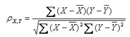
相关性值具有以下含义:
- -1.0:完全负相关
- 0.0:不相关
- 1.0:完全正相关
相关系数的绝对值越大,相关性越强,相关系数越接近于1或-1,相关度越强,相关系数越接近于0,相关度越弱。
当两个变量的标准差都不为零时,相关系数才有定义,皮尔逊相关系数适用于:
(1)、两个变量之间是线性关系,都是连续数据。
(2)、两个变量的总体是正态分布,或接近正态的单峰分布。
(3)、两个变量的观测值是成对的,每对观测值之间相互独立。
correlation_dataframe = training_examples.copy()
correlation_dataframe["target"] = training_targets["median_house_value"]
#显示各特征值之间的相关系数
correlation_dataframe.corr()

理想情况下,我们希望具有与目标密切相关的特征。
此外,我们还希望有一些相互之间的相关性不太密切的特征,以便它们添加独立信息。
在这里设置了两个特征值
#被注释掉的是我自己挑选的两个特征,其中minimal_features是与target关系最强的特征,而total_bedrooms是与minimal_features的相关系数为0的特征,没有注释的是解决方案的内容
#minimal_features = ["median_income", "total_bedrooms",]
minimal_features = [
  "median_income",
  "latitude",
]
minimal_training_examples = training_examples[minimal_features]
minimal_validation_examples = validation_examples[minimal_features]

_ = train_model(
    learning_rate=0.01,
    steps=500,
    batch_size=5,
    training_examples=minimal_training_examples,
    training_targets=training_targets,
    validation_examples=minimal_validation_examples,
    validation_targets=validation_targets)
我的选择:

解决方案:

任务 2:更好地利用纬度
绘制 latitude 与 median_house_value 的图形后,表明两者确实不存在线性关系。
不过,有几个峰值与洛杉矶和旧金山大致相对应。
plt.scatter(training_examples["latitude"], training_targets["median_house_value"])

尝试创建一些能够更好地利用纬度的合成特征。
例如,您可以创建某个特征,将 latitude 映射到值 |latitude - 38|,并将该特征命名为 distance_from_san_francisco。
或者,您可以将该空间分成 10 个不同的分桶(例如 latitude_32_to_33、latitude_33_to_34 等):如果 latitude 位于相应分桶范围内,则显示值 1.0;如果不在范围内,则显示值 0.0。
使用相关矩阵来指导您构建合成特征;如果您发现效果还不错的合成特征,可以将其添加到您的模型中。
#这里由于python2返回的是列表数组,而python3中返回的是元组,需要改正语句
#LATITUDE_RANGES = zip(range(32, 44), range(33, 45))

LATITUDE_RANGES = [(32, 33), (33, 34), (34, 35), (35, 36), (36, 37), (37, 38), (38, 39), (39, 40), (40, 41), (41, 42), (42, 43), (43, 44)]

def select_and_transform_features(source_df):
  selected_examples = pd.DataFrame()
  selected_examples["median_income"] = source_df["median_income"]
  #在不同的箱子中对需要分布的特值进行分布,在这里使用的是匿名语句lambda,判断当前特征值是否处在此箱中
  for r in LATITUDE_RANGES:
    selected_examples["latitude_%d_to_%d" % r] = source_df["latitude"].apply(
      lambda l: 1.0 if l >= r[0] and l < r[1] else 0.0)
  display.display(selected_examples.tail())
  return selected_examples

selected_training_examples = select_and_transform_features(training_examples)
selected_validation_examples = select_and_transform_features(validation_examples)

_ = train_model(
    learning_rate=0.01,
    steps=500,
    batch_size=5,
    training_examples=selected_training_examples,
    training_targets=training_targets,
    validation_examples=selected_validation_examples,
    validation_targets=validation_targets)

