预设置
from __future__ import print_function

import math

from IPython import display
from matplotlib import cm
from matplotlib import gridspec
from matplotlib import pyplot as plt
import numpy as np
import pandas as pd
from sklearn import metrics
import tensorflow as tf
from tensorflow.python.data import Dataset

tf.logging.set_verbosity(tf.logging.ERROR)
#设置最大显示行数为10
pd.options.display.max_rows = 10
#设置显示浮点数格式为一位小数
pd.options.display.float_format = '{:.1f}'.format
#导入数据
california_housing_dataframe = pd.read_csv("https://download.mlcc.google.cn/mledu-datasets/california_housing_train.csv", sep=",")
#数据随机打乱
#california_housing_dataframe = california_housing_dataframe.reindex(
#   np.random.permutation(california_housing_dataframe.index))
函数定义:特征预处理函数与标签预处理函数
def preprocess_features(california_housing_dataframe):
  """Prepares input features from California housing data set.

  Args:
    california_housing_dataframe: A Pandas DataFrame expected to contain data
      from the California housing data set.
  Returns:
    A DataFrame that contains the features to be used for the model, including
    synthetic features.
  """
  #设置选取的特征
  selected_features = california_housing_dataframe[
    ["latitude",
     "longitude",
     "housing_median_age",
     "total_rooms",
     "total_bedrooms",
     "population",
     "households",
     "median_income"]]
  #拷贝一份
  processed_features = selected_features.copy()
  # Create a synthetic feature.
  #设置一个新的合成特征
  processed_features["rooms_per_person"] = (
    california_housing_dataframe["total_rooms"] /
    california_housing_dataframe["population"])
  #特征预处理完毕
  return processed_features
#标签预处理函数
def preprocess_targets(california_housing_dataframe):
  """Prepares target features (i.e., labels) from California housing data set.
  Args:
    california_housing_dataframe: A Pandas DataFrame expected to contain data
      from the California housing data set.
  Returns:
    A DataFrame that contains the target feature.
  """
  #设置一个新的空DataFrame用于存储标签数据
  output_targets = pd.DataFrame()
  # Scale the target to be in units of thousands of dollars.
  #预设置
  output_targets["median_house_value"] = (
    california_housing_dataframe["median_house_value"] / 1000.0)
  return output_targets
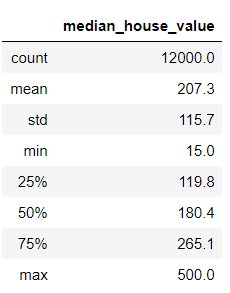
对于训练集,我们从共 17000 个样本中选择前 12000 个样本。
#在特征数据中将前12000个数据取出用来进行训练
training_examples = preprocess_features(california_housing_dataframe.head(12000))
training_examples.describe()
training_targets = preprocess_targets(california_housing_dataframe.head(12000))
training_targets.describe()

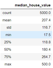
对于验证集,我们从共 17000 个样本中选择后 5000 个样本。
validation_examples = preprocess_features(california_housing_dataframe.tail(5000))
validation_examples.describe()
validation_targets = preprocess_targets(california_housing_dataframe.tail(5000))
validation_targets.describe()

任务 1:检查数据
好的,我们看一下上面的数据。可以使用的输入特征有 9 个。
快速浏览一下表格中的值。一切看起来正常吗?看一下您可以发现多少问题。如果您没有统计学方面的背景知识,也不必担心;您可以运用常识。
我们根据基准预期情况检查一下我们的数据:
对于一些值(例如 median_house_value),我们可以检查这些值是否位于合理的范围内(请注意,这是 1990 年的数据,不是现在的!)。
对于 latitude 和 longitude 等其他值,我们可以通过 Google 进行快速搜索,并快速检查一下它们与预期值是否一致。
如果您仔细看,可能会发现下列异常情况:
median_income 位于 3 到 15 的范围内。我们完全不清楚此范围究竟指的是什么,看起来可能是某对数尺度?无法找到相关记录;我们所能假设的只是,值越高,相应的收入越高。
median_house_value 的最大值是 500.0。这看起来像是某种人为设定的上限。
rooms_per_person 特征通常在正常范围内,其中第 75 百分位数的值约为 2。但也有一些非常大的值(例如 18 或 55),这可能表明数据有一定程度的损坏。
任务 2:绘制纬度/经度与房屋价值中位数的曲线图
我们来详细了解一下 latitude 和 longitude 这两个特征。它们是相关城市街区的地理坐标。
利用这两个特征可以提供出色的可视化结果 - 我们来绘制 latitude 和 longitude 的曲线图,然后用颜色标注 median_house_value。
#设置绘图参数
plt.figure(figsize=(13, 8))
ax = plt.subplot(1, 2, 1)
ax.set_title("Validation Data")
#取消自动缩放
ax.set_autoscaley_on(False)
#设置范围
ax.set_ylim([32, 43])
ax.set_autoscalex_on(False)
ax.set_xlim([-126, -112])
#绘制散点图:x轴为经度y轴为纬度,颜色图谱为冷暖色,颜色数值为房价
plt.scatter(validation_examples["longitude"],
            validation_examples["latitude"],
            cmap="coolwarm",
            c=validation_targets["median_house_value"] / validation_targets["median_house_value"].max())

ax = plt.subplot(1,2,2)
ax.set_title("Training Data")

ax.set_autoscaley_on(False)
ax.set_ylim([32, 43])
ax.set_autoscalex_on(False)
ax.set_xlim([-126, -112])
plt.scatter(training_examples["longitude"],
            training_examples["latitude"],
            cmap="coolwarm",
            c=training_targets["median_house_value"] / training_targets["median_house_value"].max())
_ = plt.plot()

如果我们的训练是成功的,那么训练集与验证集的分布应该是大致一致的,但是很明显这两个图案并不一致,甚至两个图案其实可以拼接起来看成一个数据集给出的数据
这一事实表明我们创建训练集和验证集的拆分方式很可能存在问题。为什么会导致这个结果呢?
任务 3:返回来看数据导入和预处理代码,看一下您是否发现了任何错误
在这一步中,我们会学到一项重要经验。
机器学习中的调试通常是数据调试而不是代码调试。 如果数据有误,即使最高级的机器学习代码也挽救不了局面。
返回上面的代码我们会发现:
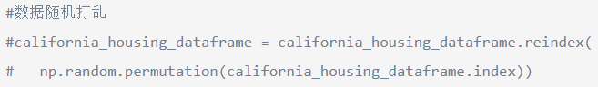
这段代码被我们注释掉了,而没有进行随机打乱的数据集由于其中可能带有部分关系或者顺序,其给出的最终结果当然就少了很多的说服力
我们解除注释再试一试

这次的分布就比较符合预期了
任务 4:训练和评估模型
我们来定义一下以前将数据加载到 TensorFlow 模型中时所使用的同一输入函数。
def my_input_fn(features, targets, batch_size=1, shuffle=True, num_epochs=None):
    """Trains a linear regression model of multiple features.

    Args:
      features: pandas DataFrame of features
      targets: pandas DataFrame of targets
      batch_size: Size of batches to be passed to the model(传递给模型的批次大小)
      shuffle: True or False. Whether to shuffle the data.(对或错。 是否随机传递数据)
      num_epochs: Number of epochs for which data should be repeated. (应重复数据的周期数。)None = repeat indefinitely
    Returns:
      Tuple of (features, labels) for next data batch(返回的是一个元组,以特征,标签组成)
    """

    # Convert pandas data into a dict of np arrays.
    # dict(features).items():将输入的特征值转换为dictinary(python的一种数据类型),通过for语句遍历,得到其所有的一一对应的值(key:value)
    features = {key:np.array(value) for key,value in dict(features).items()}

    # Construct a dataset, and configure batching/repeating.
	# Dataset.from_tensor_slices((features,targets))将输入的两个参数拼接组合起来(feature1,target1),(feature2,target2)
    ds = Dataset.from_tensor_slices((features,targets)) # warning: 2GB limit
    # 将ds数据集按照batch_size大小组合成一个batch并以num_epochs的周期重复读取下去
    ds = ds.batch(batch_size).repeat(num_epochs)

    # Shuffle the data, if specified.
    # 现在ds中的数据集已经时按照batchsize组合成得一个一个batch,存放在队列中,并且重复了n次,这样子的话,不断重复,后面数据没有意义,所以将其随机打乱,每次取出butter_size的大小
 if shuffle:
      ds = ds.shuffle(buffer_size=10000)

    # Return the next batch of data.返回下一批数据
    # make_one_shot_iterator().get_next():用迭代器迭代并在执行过程中返回所有的结果
    features, labels = ds.make_one_shot_iterator().get_next()
    return features, labels
由于我们现在使用的是多个输入特征,因此需要把用于将特征列配置为独立函数的代码模块化。(目前此代码相当简单,因为我们的所有特征都是数值,但当我们在今后的练习中使用其他类型的特征时,会基于此代码进行构建。)
def construct_feature_columns(input_features):
  """Construct the TensorFlow Feature Columns.

  Args:
    input_features: The names of the numerical input features to use.
  Returns:
    A set of feature columns
  """
  return set([tf.feature_column.numeric_column(my_feature)
              for my_feature in input_features])
接下来,继续完成下面的 train_model() 代码,以设置输入函数和计算预测。
注意:可以参考以前的练习中的代码,但要确保针对相应数据集调用 predict()。Google 机器学习编程笔记二——第一次构建线性回归模型
比较训练数据和验证数据的损失。使用一个原始特征时,我们得到的最佳均方根误差 (RMSE) 约为 180。
现在我们可以使用多个特征,不妨看一下可以获得多好的结果。
使用我们之前了解的一些方法检查数据。这些方法可能包括:
比较预测值和实际目标值的分布情况
绘制预测值和目标值的散点图
使用 latitude 和 longitude 绘制两个验证数据散点图:
一个散点图将颜色映射到实际目标 median_house_value
另一个散点图将颜色映射到预测的 median_house_value,并排进行比较。
def train_model(
    learning_rate,
    steps,
    batch_size,
    training_examples,
    training_targets,
    validation_examples,
    validation_targets):
  """Trains a linear regression model of multiple features.

  In addition to training, this function also prints training progress information,
  as well as a plot of the training and validation loss over time.

  Args:
    learning_rate: A `float`, the learning rate.
    steps: A non-zero `int`, the total number of training steps. A training step
      consists of a forward and backward pass using a single batch.
    batch_size: A non-zero `int`, the batch size.
    training_examples: A `DataFrame` containing one or more columns from
      `california_housing_dataframe` to use as input features for training.
    training_targets: A `DataFrame` containing exactly one column from
      `california_housing_dataframe` to use as target for training.
    validation_examples: A `DataFrame` containing one or more columns from
      `california_housing_dataframe` to use as input features for validation.
    validation_targets: A `DataFrame` containing exactly one column from
      `california_housing_dataframe` to use as target for validation.

  Returns:
    A `LinearRegressor` object trained on the training data.
  """
  #训练集分10批进行训练
  periods = 10
  steps_per_period = steps / periods

  # Create a linear regressor object.
  #设置线性回归训练模型
  my_optimizer = tf.train.GradientDescentOptimizer(learning_rate=learning_rate)
  #设置梯度裁剪器
  my_optimizer = tf.contrib.estimator.clip_gradients_by_norm(my_optimizer, 5.0)
  #设置线性回归模型的特征列与优化器
  linear_regressor = tf.estimator.LinearRegressor(
      feature_columns=construct_feature_columns(training_examples),
      optimizer=my_optimizer
  )
  #设置输入函数
  # Create input functions.
  #把训练样本和训练目标以及批次大小导入训练输入函数
  training_input_fn = lambda: my_input_fn(
      training_examples,
      training_targets["median_house_value"],
      batch_size=batch_size)
  #把训练样本,目标,和重复周期导入训练预测函数
  predict_training_input_fn = lambda: my_input_fn(
      training_examples,
      training_targets["median_house_value"],
      num_epochs=1,
      shuffle=False)
  #把验证样本,目标,和重复周期导入验证预测函数
  predict_validation_input_fn = lambda: my_input_fn(
      validation_examples, validation_targets["median_house_value"],
      num_epochs=1,
      shuffle=False)

  # Train the model, but do so inside a loop so that we can periodically assess
  # loss metrics.
  print("Training model...")
  print("RMSE (on training data):")
  #变量:存储均方根误差的数组
  training_rmse = []
  validation_rmse = []
  #重复period次数的训练
  for period in range (0, periods):
    # Train the model, starting from the prior state.
    #使用训练输入函数输入训练集,从上一次停止位置继续(停下来输出训练过程中的数据)
    linear_regressor.train(
        input_fn=training_input_fn,
        steps=steps_per_period,
    )
    # Take a break and compute predictions.
    #当前训练完成后将预测内容返回
    training_predictions = linear_regressor.predict(input_fn=predict_training_input_fn)
    #将预测返回的pandas特征数据提取成numpy列表数组,下验证集方式同样
    training_predictions = np.array([item['predictions'][0] for item in training_predictions])
    validation_predictions = linear_regressor.predict(input_fn=predict_validation_input_fn)
    validation_predictions = np.array([item['predictions'][0] for item in validation_predictions])
    # Compute training and validation loss.
    #计算均方根误差
    training_root_mean_squared_error = math.sqrt(
        metrics.mean_squared_error(training_predictions, training_targets))
    validation_root_mean_squared_error = math.sqrt(
        metrics.mean_squared_error(validation_predictions, validation_targets))
    # Occasionally print the current loss.
    print("  period %02d : %0.2f" % (period, training_root_mean_squared_error))
    # 将当前的均方根误差存储到总数组中,用于训练跑完之后画出曲线图
    # Add the loss metrics from this period to our list.
    training_rmse.append(training_root_mean_squared_error)
    validation_rmse.append(validation_root_mean_squared_error)
  print("Model training finished.")
  #画图
  # Output a graph of loss metrics over periods.
  plt.ylabel("RMSE")
  plt.xlabel("Periods")
  plt.title("Root Mean Squared Error vs. Periods")
  plt.tight_layout()
  plt.plot(training_rmse, label="training")
  plt.plot(validation_rmse, label="validation")
  plt.legend()

  return linear_regressor

任务 5:基于测试数据进行评估
在以下单元格中,载入测试数据集并据此评估模型。
我们已对验证数据进行了大量迭代。接下来确保我们没有过拟合该特定样本集的特性。
california_housing_test_data = pd.read_csv("https://download.mlcc.google.cn/mledu-datasets/california_housing_test.csv", sep=",")

test_examples = preprocess_features(california_housing_test_data)
test_targets = preprocess_targets(california_housing_test_data)

predict_test_input_fn = lambda: my_input_fn(
      test_examples,
      test_targets["median_house_value"],
      num_epochs=1,
      shuffle=False)

test_predictions = linear_regressor.predict(input_fn=predict_test_input_fn)
test_predictions = np.array([item['predictions'][0] for item in test_predictions])

root_mean_squared_error = math.sqrt(
    metrics.mean_squared_error(test_predictions, test_targets))

print("Final RMSE (on test data): %0.2f" % root_mean_squared_error)
总之我们在这里的步骤大致为:
1、设置训练集,验证集,测试集,其中每个都要设置出数据集与目标集
2、定义预处理函数,将我们可能使用到的特征提取出来,若有需要的合成特征也进行合成
3、定义输入函数,设置需要进行迭代的批数等,返回需要的(特征,标签)元组
注意: 在这里如果特征较多还需要定义一个特征函数,将需要的特征列组成一个集合返回
4、分批预测,输出结果
