本文介绍fminunc的使用,结合bfgs的例子一起说一说、
关于BFGS的用法,自己找资料看一下原理,基本上意思就是用一个近似的方法将原有的Hessian矩阵替代掉:下面的截图来自陆吾生老师:

验证下来BFGS要比DFP收敛效果更好。Matlab里面我们举例子就用BFGS
我们现在给出优化函数:
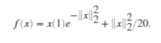
去这个函数的最小值,不带任何约束。
写成func@ 的形式
fun = @(x)x(1)*exp(-(x(1)^2 + x(2)^2)) + (x(1)^2 + x(2)^2)/20;
然后我们还要设置一个初始值
x0 = [1,2];
最后直接调用fminunc求解:
[x,fval] = fminunc(fun,x0)
能够获得的信息就是最后的最后的函数最优点和函数值,以及迭代次数等
Local minimum found.

Optimization completed because the size of the gradient is less than
the value of the optimality tolerance.

<stopping criteria details>

x =

   -0.6691    0.0000


fval =

   -0.4052


exitflag =

     1


output =

  struct with fields:

       iterations: 9
        funcCount: 42
         stepsize: 2.9345e-04
     lssteplength: 1
    firstorderopt: 8.0839e-07
        algorithm: 'quasi-newton'
          message: '↵Local minimum found.↵↵Optimization completed because the size of the gradient is less than↵the value of the optimality tolerance.↵↵<stopping criteria details>↵↵Optimization completed: The first-order optimality measure, 6.891345e-07, is less ↵than options.OptimalityTolerance = 1.000000e-06.↵↵'
但是,为了获得更多的结算信息,我们可以根据上一个博客中提到的set parameter的方法,加入一个options人工的添加一些你感兴趣的信息来显示:
clc
clear all

options = optimoptions(@fminunc,'Display','iter','Algorithm','quasi-newton');
 fun = @(x)x(1)*exp(-(x(1)^2 + x(2)^2)) + (x(1)^2 + x(2)^2)/20;
%fun = @(x)3*x(1)^2 + 2*x(1)*x(2) + x(2)^2 - 4*x(1) + 5*x(2);
x0 = [1,2];
[x,fval,exitflag,output] = fminunc(fun,x0,options)
结果是:
                                                     First-order
 Iteration  Func-count       f(x)        Step-size       optimality
     0           3         0.256738                         0.173
     1           6         0.222149              1          0.131
     2           9          0.15717              1          0.158
     3          18        -0.227902       0.438133          0.386
     4          21        -0.299271              1           0.46
     5          30        -0.404028       0.102071         0.0458
     6          33        -0.404868              1         0.0296
     7          36        -0.405236              1        0.00119
     8          39        -0.405237              1       0.000252
     9          42        -0.405237              1       8.08e-07

Local minimum found.

Optimization completed because the size of the gradient is less than
the value of the optimality tolerance.

<stopping criteria details>

x =

   -0.6691    0.0000


fval =

   -0.4052


exitflag =

     1


output =

  struct with fields:

       iterations: 9
        funcCount: 42
         stepsize: 2.9345e-04
     lssteplength: 1
    firstorderopt: 8.0839e-07
        algorithm: 'quasi-newton'
          message: '↵Local minimum found.↵↵Optimization completed because the size of the gradient is less than↵the value of the optimality tolerance.↵↵<stopping criteria details>↵↵Optimization completed: The first-order optimality measure, 6.891345e-07, is less ↵than options.OptimalityTolerance = 1.000000e-06.↵↵'

>>
我们在这里就获得了更多地迭代过程中的中间信息。
另外一种写法,依然是使用一个例子来说明:

要最小化以上函数:
clc
clear all

options = optimoptions('fminunc','Display','iter','Algorithm','quasi-newton');
problem.options = options;
problem.x0 = [1;2];
problem.objective = @func;
problem.solver = 'fminunc';
x = fminunc(problem)
设置了使用拟牛顿法求解:
                                                        First-order
 Iteration  Func-count       f(x)        Step-size       optimality
     0           3              100                           400
     1           9         0.164722    0.000892027           11.2
     2          12         0.131169              1           4.88
     3          15         0.122653              1          0.242
     4          21           0.1222             10          0.528
     5          24         0.120055              1           1.65
     6          27         0.113967              1           3.75
     7          30         0.104296              1           6.04
     8          33        0.0909524              1           7.19
     9          36        0.0657965              1           6.56
    10          39        0.0337093              1           2.53
    11          42        0.0195464              1           3.87
    12          45       0.00649517              1          0.422
    13          51       0.00315672       0.660962           1.58
    14          54       0.00103291              1          0.767
    15          57      0.000151308              1          0.238
    16          60       1.3137e-05              1          0.114
    17          63      6.02652e-06              1         0.0868
    18          66      2.77992e-07              1        0.00588
    19          69       1.0918e-09              1       0.000443
                                                        First-order
 Iteration  Func-count       f(x)        Step-size       optimality
    20          72      2.30071e-11              1          4e-05

Local minimum found.

Optimization completed because the size of the gradient is less than
the value of the optimality tolerance.

<stopping criteria details>

x =

    1.0000
    1.0000

>>
当然我们还可以使用置信区间法求解,这里要求设置梯度为真:
clc
clear all
 options = optimoptions('fminunc','Display','iter','Algorithm','trust-region','SpecifyObjectiveGradient',true);
% options = optimoptions('fminunc','Display','iter','Algorithm','quasi-newton');
problem.options = options;
problem.x0 = [1;2];
problem.objective = @func;
problem.solver = 'fminunc';
x = fminunc(problem)

function [f,g] = func(x)
% Calculate objective f
f = 100*(x(2) - x(1)^2)^2 + (1-x(1))^2;

if nargout > 1 % gradient required
    g = [-400*(x(2)-x(1)^2)*x(1)-2*(1-x(1));
        200*(x(2)-x(1)^2)];
end
end
我们为了使用梯度,引入了一个自己写的函数fun, 这里面包括了函数本身以及他的梯度,在options里面我们也设置了相关使用梯度的参数:“‘trust-region’,‘SpecifyObjectiveGradient’,true);”,要注意这里如果使用置信区间那就必须要使用梯度,两者要同时出现。
结果如下:
                                Norm of      First-order
 Iteration        f(x)          step          optimality   CG-iterations
     0                100                           400
     1                100             10            400           1
     2                100            2.5            400           0
     3            27.8984          0.625            341           0
     4           0.374736       0.505714           1.25           1
     5            0.29229          0.625           19.8           1
     6           0.138484        0.13794           2.45           1
     7           0.138484       0.663579           2.45           1
     8           0.100293        0.15625           1.74           0
     9          0.0560498         0.3125           6.18           1
    10          0.0220561       0.145628           1.94           1
    11         0.00854943       0.205656           3.09           1
    12         0.00128111      0.0527322          0.332           1
    13        0.000111288      0.0713324          0.401           1
    14         4.3117e-07     0.00656459        0.00568           1
    15         1.9432e-11     0.00143547        0.00017           1

Local minimum possible.

fminunc stopped because the final change in function value relative to
its initial value is less than the value of the function tolerance.

<stopping criteria details>

x =

    1.0000
    1.0000

>>
