本章节研究内容：词向量介绍＋word2vec两种架构cbow&skip-gram＋google word2vec 源码分析＋滑动窗口如何构建数据

词向量表示

One-Hot Representation

NLP 中最直观，也是到目前为止最常用的词表示方法是 One-hot Representation，这种方法把每个词表示为一个很长的向量。这个向量的维度是词表大小，其中绝大多数元素为 0，只有一个维度的值为 1，这个维度就代表了当前的词。

举个栗子，

“话筒”表示为 [0 0 0 1 0 0 0 0 0 0 0 0 0 0 0 0 …]

“麦克”表示为 [0 0 0 0 0 0 0 0 1 0 0 0 0 0 0 0 …]

每个词都是茫茫 0 海中的一个 1。
这种 One-hot Representation 如果采用稀疏方式存储，会是非常的简洁：也就是给每个词分配一个数字 ID。比如刚才的例子中，话筒记为 3，麦克记为 8（假设从 0 开始记）。

问题：无法获取词与词之间的相似度；维数多个，稀疏严重

Distributed Represetation

Deep Learning 中一般用到的词向量是用 Distributed Representation表示的一种低维实数向量。例如： [0.792, −0.177, −0.107, 0.109, −0.542, …]。维度以 50 维和 100 维比较常见

通过训练将每个词映射K维的向量，可以通过词语间矩阵（例如： cos）来判断语义相似度。而Word2Vec 使用这种方式表示。
用这种方式表示的向量，“麦克”和“话筒”的距离会远远小于“麦克”和“天气”。

Distributed representation 用来表示词，通常被称为“Word Representation”或“Word Embedding”，中文俗称“词向量”。

语言模型训练

初步介绍

找常出现在每个单词附近的词，就能获得它们的映射关系.步骤如下：

先是获取大量文本数据(例如所有维基百科内容)
然后我们建立一个可以沿文本滑动的窗(例如一个窗里包含三个单词)
利用这样的滑动窗就能为训练模型生成大量样本数据。

窗口滑动，生成模型训练的数据集，通过下面的进行演示

窗口锁定在句子的前三个单词上
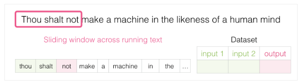
前两个单词单做特征，第三个单词单做标签：生产了数据集中的第一个样本
窗口滑动到下一个位置并生产第二个样本
所有数据集上全部滑动后，我们得到一个较大的数据集

图摘自：《Efficient Estimation of Word Representations in Vector Space.pdf》

在这里插入图片描述

CBOW 模型架构

CBOW 有两种可选的算法：层次 Softmax 和 Negative Sampling

CBOW 模型是预测 P(wt|wt-k,wt-(k-1)…,wt-1,wt+1,wt+2…,wt+k)

Softmax 算法：结合了 Huffman 编码，每个词 w 都可以从树的根结点沿着唯一一条路径被访问到；
Negative Sampling，原理说简单很简单，就是随机搞点负例。实际论文中提到按照词频的3/4 次方进行负样本的采样。

摘自google word2vec 源码： 创建Huffman tree 过程（C++)
// Create binary Huffman tree using the word counts
// Frequent words will have short uniqe binary codes
void CreateBinaryTree() {
  long long a, b, i, min1i, min2i, pos1, pos2, point[MAX_CODE_LENGTH];
  char code[MAX_CODE_LENGTH];
  long long *count = (long long *)calloc(vocab_size * 2 + 1, sizeof(long long));
  long long *binary = (long long *)calloc(vocab_size * 2 + 1, sizeof(long long));
  long long *parent_node = (long long *)calloc(vocab_size * 2 + 1, sizeof(long long));
  for (a = 0; a < vocab_size; a++) count[a] = vocab[a].cn;
  for (a = vocab_size; a < vocab_size * 2; a++) count[a] = 1e15;
  pos1 = vocab_size - 1;
  pos2 = vocab_size;
  // Following algorithm constructs the Huffman tree by adding one node at a time
  for (a = 0; a < vocab_size - 1; a++) {
    // First, find two smallest nodes 'min1, min2'
    if (pos1 >= 0) {
      if (count[pos1] < count[pos2]) {
        min1i = pos1;
        pos1--;
      } else {
        min1i = pos2;
        pos2++;
      }
    } else {
      min1i = pos2;
      pos2++;
    }
    if (pos1 >= 0) {
      if (count[pos1] < count[pos2]) {
        min2i = pos1;
        pos1--;
      } else {
        min2i = pos2;
        pos2++;
      }
    } else {
      min2i = pos2;
      pos2++;
    }
    count[vocab_size + a] = count[min1i] + count[min2i];
    parent_node[min1i] = vocab_size + a;
    parent_node[min2i] = vocab_size + a;
    binary[min2i] = 1;
  }
  // Now assign binary code to each vocabulary word
  for (a = 0; a < vocab_size; a++) {
    b = a;
    i = 0;
    while (1) {
      code[i] = binary[b];
      point[i] = b;
      i++;
      b = parent_node[b];
      if (b == vocab_size * 2 - 2) break;
    }
    vocab[a].codelen = i;
    vocab[a].point[0] = vocab_size - 2;
    for (b = 0; b < i; b++) {
      vocab[a].code[i - b - 1] = code[b];
      vocab[a].point[i - b] = point[b] - vocab_size;
    }
  }
  free(count);
  free(binary);
  free(parent_node);
}


 // 摘自 google word2vec 负采样的过程
 // NEGATIVE SAMPLING
        if (negative > 0) for (d = 0; d < negative + 1; d++) {
          if (d == 0) {
            target = word;
            label = 1;
          } else {
            next_random = next_random * (unsigned long long)25214903917 + 11;
            target = table[(next_random >> 16) % table_size];
            if (target == 0) target = next_random % (vocab_size - 1) + 1;
            if (target == word) continue;
            label = 0;
          }
          l2 = target * layer1_size;
          f = 0;
          for (c = 0; c < layer1_size; c++) f += neu1[c] * syn1neg[c + l2];
          if (f > MAX_EXP) g = (label - 1) * alpha;
          else if (f < -MAX_EXP) g = (label - 0) * alpha;
          else g = (label - expTable[(int)((f + MAX_EXP) * (EXP_TABLE_SIZE / MAX_EXP / 2))]) * alpha;
          for (c = 0; c < layer1_size; c++) neu1e[c] += g * syn1neg[c + l2];
          for (c = 0; c < layer1_size; c++) syn1neg[c + l2] += g * neu1[c];
        }