softmax和分类模型

内容包含：

softmax回归的基本概念（见《动手学深度学习》）
如何获取Fashion-MNIST数据集和读取数据
softmax回归模型的从零开始实现，实现一个对Fashion-MNIST训练集中的图像数据进行分类的模型
使用pytorch重新实现softmax回归模型

1.获取Fashion-MNIST训练集和读取数据

多类图像分类数据集Fashion-MNIST
torchvision包，用来构建计算机视觉模型,主要由以下几部分构成：

torchvision.datasets: 一些加载数据的函数及常用的数据集接口；
torchvision.models: 包含常用的模型结构（含预训练模型），例如AlexNet、VGG、ResNet等；
torchvision.transforms: 常用的图片变换，例如裁剪、旋转等；
torchvision.utils: 其他的一些有用的方法。

# import needed package
%matplotlib inline
from IPython import display
import matplotlib.pyplot as plt

import torch
import torchvision
import torchvision.transforms as transforms
import time

import sys
sys.path.append("/home/kesci/input")
import d2lzh1981 as d2l

print(torch.__version__)
print(torchvision.__version__)

输出
1.3.0
0.4.1a0+d94043a

## get dataset
mnist_train = torchvision.datasets.FashionMNIST(root='/home/kesci/input/FashionMNIST2065', train=True, download=True, transform=transforms.ToTensor())
mnist_test = torchvision.datasets.FashionMNIST(root='/home/kesci/input/FashionMNIST2065', train=False, download=True, transform=transforms.ToTensor())

# show result 
print(type(mnist_train))
print(len(mnist_train), len(mnist_test))

输出
<class ‘torchvision.datasets.mnist.FashionMNIST’>
60000 10000

如果不做变换输入的数据是图像，我们可以看一下图片的类型参数：

mnist_PIL = torchvision.datasets.FashionMNIST(root='/home/kesci/input/FashionMNIST2065', train=True, download=True)
PIL_feature, label = mnist_PIL[0]
print(PIL_feature)

输出
<PIL.Image.Image image mode=L size=28x28 at 0x7F085198D9E8>

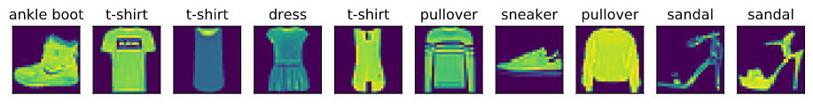
# 本函数已保存在d2lzh包中方便以后使用
def get_fashion_mnist_labels(labels):
    text_labels = ['t-shirt', 'trouser', 'pullover', 'dress', 'coat',
                   'sandal', 'shirt', 'sneaker', 'bag', 'ankle boot']
    return [text_labels[int(i)] for i in labels]

def show_fashion_mnist(images, labels):
    d2l.use_svg_display()
    # 这里的_表示我们忽略（不使用）的变量
    _, figs = plt.subplots(1, len(images), figsize=(12, 12))
    for f, img, lbl in zip(figs, images, labels):
        f.imshow(img.view((28, 28)).numpy())
        f.set_title(lbl)
        f.axes.get_xaxis().set_visible(False)
        f.axes.get_yaxis().set_visible(False)
    plt.show()

X, y = [], []
for i in range(10):
    X.append(mnist_train[i][0]) # 将第i个feature加到X中
    y.append(mnist_train[i][1]) # 将第i个label加到y中
show_fashion_mnist(X, get_fashion_mnist_labels(y))

输出
在这里插入图片描述

# 读取数据
batch_size = 256
num_workers = 4
train_iter = torch.utils.data.DataLoader(mnist_train, batch_size=batch_size, shuffle=True, num_workers=num_workers)
test_iter = torch.utils.data.DataLoader(mnist_test, batch_size=batch_size, shuffle=False, num_workers=num_workers)

2. softmax从零开始的实现

import torch
import torchvision
import numpy as np
import sys
sys.path.append("/home/kesci/input")
import d2lzh1981 as d2l

print(torch.__version__)
print(torchvision.__version__)

#获取训练集数据和测试集数据
batch_size = 256
train_iter, test_iter = d2l.load_data_fashion_mnist(batch_size, root='/home/kesci/input/FashionMNIST2065')

#模型参数初始化
num_inputs = 784
print(28*28)
num_outputs = 10

W = torch.tensor(np.random.normal(0, 0.01, (num_inputs, num_outputs)), dtype=torch.float)
b = torch.zeros(num_outputs, dtype=torch.float)

W.requires_grad_(requires_grad=True)
b.requires_grad_(requires_grad=True)

# 对多维Tensor按维度操作
X = torch.tensor([[1, 2, 3], [4, 5, 6]])
print(X.sum(dim=0, keepdim=True))  # dim为0，按照相同的列求和，并在结果中保留列特征
print(X.sum(dim=1, keepdim=True))  # dim为1，按照相同的行求和，并在结果中保留行特征
print(X.sum(dim=0, keepdim=False)) # dim为0，按照相同的列求和，不在结果中保留列特征
print(X.sum(dim=1, keepdim=False)) # dim为1，按照相同的行求和，不在结果中保留行特征

tensor([[5, 7, 9]])
tensor([[ 6],
[15]])
tensor([5, 7, 9])
tensor([ 6, 15])

定义softmax操作

$\hat{y}_j = \frac{ \exp(o_j)}{\sum_{i=1}^3 \exp(o_i)}$

def softmax(X):
    X_exp = X.exp()
    partition = X_exp.sum(dim=1, keepdim=True)
    # print("X size is ", X_exp.size())
    # print("partition size is ", partition, partition.size())
    return X_exp / partition  # 这里应用了广播机制

X = torch.rand((2, 5))
X_prob = softmax(X)
print(X_prob, '\n', X_prob.sum(dim=1))

tensor([[0.2441, 0.2439, 0.1263, 0.1885, 0.1972],
[0.2408, 0.1987, 0.1400, 0.1199, 0.3006]])
tensor([1.0000, 1.0000])

softmax回归模型

$\begin{aligned} \boldsymbol{o}^{(i)} &= \boldsymbol{x}^{(i)} \boldsymbol{W} + \boldsymbol{b},\\ \boldsymbol{\hat{y}}^{(i)} &= \text{softmax}(\boldsymbol{o}^{(i)}). \end{aligned}$

def net(X):
    return softmax(torch.mm(X.view((-1, num_inputs)), W) + b)

定义损失函数

$H\left(\boldsymbol y^{(i)}, \boldsymbol {\hat y}^{(i)}\right ) = -\sum_{j=1}^q y_j^{(i)} \log \hat y_j^{(i)},$

$\ell(\boldsymbol{\Theta}) = \frac{1}{n} \sum_{i=1}^n H\left(\boldsymbol y^{(i)}, \boldsymbol {\hat y}^{(i)}\right ),$

$\ell(\boldsymbol{\Theta}) = -(1/n) \sum_{i=1}^n \log \hat y_{y^{(i)}}^{(i)}$

y_hat = torch.tensor([[0.1, 0.3, 0.6], [0.3, 0.2, 0.5]])
y = torch.LongTensor([0, 2])
y_hat.gather(1, y.view(-1, 1))

tensor([[0.1000],
[0.5000]])

def cross_entropy(y_hat, y):
    return - torch.log(y_hat.gather(1, y.view(-1, 1)))

定义准确率

def accuracy(y_hat, y):
    return (y_hat.argmax(dim=1) == y).float().mean().item()

print(accuracy(y_hat, y))

0.5

# 本函数已保存在d2lzh_pytorch包中方便以后使用。该函数将被逐步改进：它的完整实现将在“图像增广”一节中描述
def evaluate_accuracy(data_iter, net):
    acc_sum, n = 0.0, 0
    for X, y in data_iter:
        acc_sum += (net(X).argmax(dim=1) == y).float().sum().item()
        n += y.shape[0]
    return acc_sum / n

print(evaluate_accuracy(test_iter, net))

0.0745

训练模型

num_epochs, lr = 5, 0.1

# 本函数已保存在d2lzh_pytorch包中方便以后使用
def train_ch3(net, train_iter, test_iter, loss, num_epochs, batch_size,
              params=None, lr=None, optimizer=None):
    for epoch in range(num_epochs):
        train_l_sum, train_acc_sum, n = 0.0, 0.0, 0
        for X, y in train_iter:
            y_hat = net(X)
            l = loss(y_hat, y).sum()
            
            # 梯度清零
            if optimizer is not None:
                optimizer.zero_grad()
            elif params is not None and params[0].grad is not None:
                for param in params:
                    param.grad.data.zero_()
            
            l.backward()
            if optimizer is None:
                d2l.sgd(params, lr, batch_size)
            else:
                optimizer.step() 
            
            
            train_l_sum += l.item()
            train_acc_sum += (y_hat.argmax(dim=1) == y).sum().item()
            n += y.shape[0]
        test_acc = evaluate_accuracy(test_iter, net)
        print('epoch %d, loss %.4f, train acc %.3f, test acc %.3f'
              % (epoch + 1, train_l_sum / n, train_acc_sum / n, test_acc))

train_ch3(net, train_iter, test_iter, cross_entropy, num_epochs, batch_size, [W, b], lr)

epoch 1, loss 0.7870, train acc 0.746, test acc 0.792
epoch 2, loss 0.5707, train acc 0.813, test acc 0.814
epoch 3, loss 0.5242, train acc 0.826, test acc 0.819
epoch 4, loss 0.5017, train acc 0.832, test acc 0.825
epoch 5, loss 0.4848, train acc 0.837, test acc 0.828

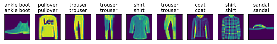
模型预测

模型训练完，进行预测。
给定一系列图像（第三行图像输出），比较它们的真实标签（第一行文本输出）和模型预测结果（第二行文本输出）。

X, y = iter(test_iter).next()

true_labels = d2l.get_fashion_mnist_labels(y.numpy())
pred_labels = d2l.get_fashion_mnist_labels(net(X).argmax(dim=1).numpy())
titles = [true + '\n' + pred for true, pred in zip(true_labels, pred_labels)]

d2l.show_fashion_mnist(X[0:9], titles[0:9])

在这里插入图片描述

3. softmax的简洁实现

# 加载各种包或者模块
import torch
from torch import nn
from torch.nn import init
import numpy as np
import sys
sys.path.append("/home/kesci/input")
import d2lzh1981 as d2l

print(torch.__version__)

初始化参数和获取数据

batch_size = 256
train_iter, test_iter = d2l.load_data_fashion_mnist(batch_size, root='/home/kesci/input/FashionMNIST2065')

定义网络模型

num_inputs = 784
num_outputs = 10

class LinearNet(nn.Module):
    def __init__(self, num_inputs, num_outputs):
        super(LinearNet, self).__init__()
        self.linear = nn.Linear(num_inputs, num_outputs)
    def forward(self, x): # x 的形状: (batch, 1, 28, 28)
        y = self.linear(x.view(x.shape[0], -1))
        return y
    
# net = LinearNet(num_inputs, num_outputs)

class FlattenLayer(nn.Module):
    def __init__(self):
        super(FlattenLayer, self).__init__()
    def forward(self, x): # x 的形状: (batch, *, *, ...)
        return x.view(x.shape[0], -1)

from collections import OrderedDict
net = nn.Sequential(
        # FlattenLayer(),
        # LinearNet(num_inputs, num_outputs) 
        OrderedDict([
           ('flatten', FlattenLayer()),
           ('linear', nn.Linear(num_inputs, num_outputs))]) # 或者写成我们自己定义的 LinearNet(num_inputs, num_outputs) 也可以
        )

初始化模型参数

init.normal_(net.linear.weight, mean=0, std=0.01)
init.constant_(net.linear.bias, val=0)

Parameter containing:
tensor([0., 0., 0., 0., 0., 0., 0., 0., 0., 0.], requires_grad=True)

定义损失函数

loss = nn.CrossEntropyLoss() # 下面是他的函数原型
# class torch.nn.CrossEntropyLoss(weight=None, size_average=None, ignore_index=-100, reduce=None, reduction='mean')

定义优化函数

optimizer = torch.optim.SGD(net.parameters(), lr=0.1) # 下面是函数原型
# class torch.optim.SGD(params, lr=, momentum=0, dampening=0, weight_decay=0, nesterov=False)

训练

num_epochs = 5
d2l.train_ch3(net, train_iter, test_iter, loss, num_epochs, batch_size, None, None, optimizer)

epoch 1, loss 0.0031, train acc 0.750, test acc 0.746
epoch 2, loss 0.0022, train acc 0.813, test acc 0.810
epoch 3, loss 0.0021, train acc 0.825, test acc 0.814
epoch 4, loss 0.0020, train acc 0.832, test acc 0.820
epoch 5, loss 0.0019, train acc 0.836, test acc 0.804

A_first

发布了1 篇原创文章 · 获赞 0 · 访问量 18

私信关注

1.2softmax和分类模型

softmax和分类模型

1.获取Fashion-MNIST训练集和读取数据

2. softmax从零开始的实现

定义softmax操作

softmax回归模型

定义损失函数

定义准确率

训练模型

模型预测

3. softmax的简洁实现

初始化参数和获取数据

定义网络模型

初始化模型参数

定义损失函数

定义优化函数

训练

猜你喜欢