版权声明:本文为CSDN博主「爱弹ukulele的程序猿」的原创文章,遵循 CC 4.0 BY-SA 版权协议,转载请附上原文出处链接及本声明。
原文链接:https://blog.csdn.net/qq_38622495/article/details/82289814
笔记目录
1 Inference
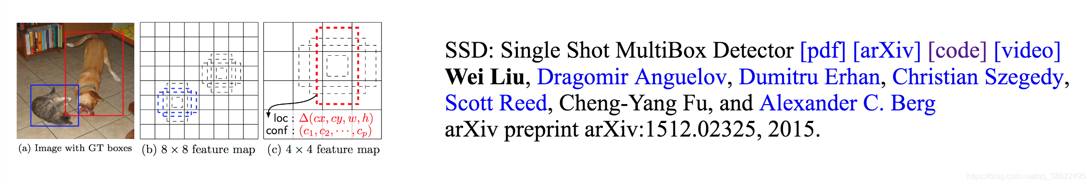
Single shot指明了SSD算法属于one-stage方法,MultiBox指明了SSD是多框预测。
SSD是一种one-stage方法,其主要思路是均匀地在图片的不同位置进行密集抽样,抽样时可以采用不同尺度和长宽比,然后利用CNN提取特征后直接进行分类与回归,整个过程只需要一步,所以其优势是速度快。
2 基本结构与设计理念
2.1 default box & feature map cell
- feature map cell 就是将 feature map 切分成
γ 可以减小正类预测值比较大时的损失。
2.2.4.3 SSD在6个层级上进行回归
3 总结
4 SSD的Gluon实现
4.1 类别预测
- 假设物体有
n类,则需要对锚框作n+1个分类,其中类0表示背景。以输入像素为中心输入a个锚框,设高、宽分别为h、w,会有a*h*w个预测结果。 - 使用卷积层的通道来输出类别预测。如果使用全连接层作为输出,可能会导致有过多的模型参数。NIN
类别预测层使用一个保持输入高宽的卷积层,其输出的
(x,y)像素通道里包含了以输入(x,y)像素为中心的所有锚框的类别预测。其输出通道数为a(n+1),其中通道i(n+1)是第 i 个锚框预测的背景置信度,而通道i(n+1)+j+1则是第 i 锚框预测的第 j 类物体的置信度。def cls_predictor(num_anchors, num_classes): return nn.Conv2D(num_anchors * (num_classes + 1), kernel_size=3, padding=1)- 1
- 2
- 3
定义分类器:
指定a和n后,它使用一个填充为 1 的3×3卷积层。注意到我们使用了较小的卷积窗口,它可能不能覆盖锚框定义的区域。所以我们需要保证前面的卷积层能有效的将较大的锚框区域的特征浓缩到一个3×3的窗口里。4.2 边界框预测
对每个锚框我们需要预测如何将其变换到真实的物体边界框。变换由一个长为 4 的向量来描述,分别表示左下和右上的 x、y 轴坐标偏移。与类别预测类似,这里我们同样使用一个保持高宽的卷积层来输出偏移预测,它有 4a 个输出通道,对于第 i 个锚框,它的偏移预测在
4i到4i+3这 4 个通道里。def bbox_predictor(num_anchors): return nn.Conv2D(num_anchors * 4, kernel_size=3, padding=1)- 1
- 2
4.3 合成多层的预测输出
SSD 中会在多个尺度上进行预测。由于每个尺度上的输入高宽和锚框的选取不一样,导致其形状各不相同。下面例子构造两个尺度的输入,其中第二个为第一个的高宽减半。然后构造两个类别预测层,其分别对每个输入像素构造 5 个和 3 个锚框。
def forward(x, block): block.initialize() return block(x) - 假设物体有
y1 = forward(nd.zeros((2, 8, 20, 20)), cls_predictor(5, 10))
y2 = forward(nd.zeros((2, 16, 10, 10)), cls_predictor(3, 10))
(y1.shape, y2.shape)
out:((2, 55, 20, 20), (2, 33, 10, 10))
- 1
- 2
- 3
- 4
- 5
- 6
- 7
- 8
- 9
- 10
预测的输出格式为(批量大小,通道数,高,宽)。首先将通道,即预测结果,放到最后。因为不同尺度下批量大小保持不变,所以将结果转成二维的(批量大小,高 × 宽 × 通道数)格式,方便之后的拼接。
首先将通道,即预测结果,放到最后。因为不同尺度下批量大小保持不变,所以将结果转成二维的(批量大小,高 × 宽 × 通道数)格式,方便之后的拼接。
def flatten_pred(pred):
    return pred.transpose(axes=(0, 2, 3, 1)).flatten()
- 1
- 2
- 3
拼接就是简单将在维度 1 上合并结果。
def concat_preds(preds):
    return nd.concat(*[flatten_pred(p) for p in preds], dim=1)
concat_preds([y1, y2]).shape
out:(2, 25300)
- 1
- 2
- 3
- 4
- 5
- 6
4.4 减半模块
减半模块将输入高宽减半来得到不同尺度的特征,这是通过步幅 2 的 2×2 最大池化层来完成。我们前面提到因为预测层的窗口为 3,所以我们需要额外卷积层来扩大其作用窗口来有效覆盖锚框区域。为此我们加入两个 3×3 卷积层,每个卷积层后接批量归一化层和 ReLU 激活层。这样,一个尺度上的 3×3 窗口覆盖了上一个尺度上的 10×10 窗口。
def down_sample_blk(num_filters):
    blk = nn.HybridSequential()
    for _ in range(2):
        blk.add(nn.Conv2D(num_filters, kernel_size=3, padding=1),
                nn.BatchNorm(in_channels=num_filters),
                nn.Activation('relu'))
    blk.add(nn.MaxPool2D(2))
    blk.hybridize()
    return blk
forward(nd.zeros((2, 3, 20, 20)), down_sample_blk(10)).shape
out:(2, 10, 10, 10)
- 1
- 2
- 3
- 4
- 5
- 6
- 7
- 8
- 9
- 10
- 11
- 12
- 13
- 14
4.5 主体网络
主体网络用来从原始图像抽取特征,一般会选择常用的深度卷积神经网络。一般使用了 VGG,大家也常用 ResNet 替代。本小节为了计算简单,我们构造一个小的主体网络。网络中叠加三个减半模块,输出通道数从 16 开始,之后每个模块对其翻倍。
def body_blk():
    blk = nn.HybridSequential()
    for num_filters in [16, 32, 64]:
        blk.add(down_sample_blk(num_filters))
    return blk
forward(nd.zeros((2, 3, 256, 256)), body_blk()).shape
out: (2, 64, 32, 32)
- 1
- 2
- 3
- 4
- 5
- 6
- 7
- 8
- 9
4.6 完整的模型
构建整个模型,这个模型有五个模块,每个模块对输入进行特征抽取,并且预测锚框的类和偏移。第一个模块使用主体网络,第二到四模块使用减半模块,最后一个模块则使用全局的最大池化层来将高宽降到 1。
def get_blk(i):
    if i == 0:
        blk = body_blk()
    elif i == 4:
        blk = nn.GlobalMaxPool2D()
    else:
        blk = down_sample_blk(128)
    return blk
- 1
- 2
- 3
- 4
- 5
- 6
- 7
- 8
定义每个模块前向计算。它跟之前的卷积神经网络不同在于,不仅输出卷积块的输出,而且还返回在输出上生成的锚框,以及每个锚框的类别预测和偏移预测。
def single_scale_forward(x, blk, size, ratio, cls_predictor, bbox_predictor):
    y = blk(x)
    anchor = contrib.ndarray.MultiBoxPrior(y, sizes=size, ratios=ratio)
    cls_pred = cls_predictor(y)
    bbox_pred = bbox_predictor(y)
    return (y, anchor, cls_pred, bbox_pred)
- 1
- 2
- 3
- 4
- 5
- 6
定义其输出上的锚框如何生成。比例固定成 1、2 和 0.5,但大小上则不同,用于覆盖不同的尺度。
num_anchors = 4
sizes = [[0.2, 0.272], [0.37, 0.447], [0.54, 0.619], [0.71, 0.79],
         [0.88, 0.961]]
ratios = [[1, 2, 0.5]] * 5
- 1
- 2
- 3
- 4
4.7完整模型定义
class TinySSD(nn.Block): def __init__(self, num_classes, verbose=False, **kwargs): super(TinySSD, self).__init__(**kwargs) self.num_classes = num_classes for i in range(5): setattr(self, 'blk_%d' % i, get_blk(i)) setattr(self, 'cls_%d' % i, cls_predictor(num_anchors, num_classes)) setattr(self, 'bbox_%d' % i, bbox_predictor(num_anchors))def forward(self, x): anchors, cls_preds, bbox_preds = [None] * 5, [None] * 5, [None] * 5 for i in range(5): x, anchors[i], cls_preds[i], bbox_preds[i] = single_scale_forward( x, getattr(self, 'blk_%d' % i), sizes[i], ratios[i], getattr(self, 'cls_%d' % i), getattr(self, 'bbox_%d' % i)) return (nd.concat(*anchors, dim=1), concat_preds(cls_preds).reshape( (0, -1, self.num_classes + 1)), concat_preds(bbox_preds))
net = TinySSD(num_classes=2, verbose=True)
net.initialize()
x = nd.zeros((2, 3, 256, 256))
anchors, cls_preds, bbox_preds = net(x)
print(‘output achors:’, anchors.shape)
print(‘output class predictions:’, cls_preds.shape)
print(‘output box predictions:’, bbox_preds.shape)
output achors: (1, 5444, 4)
output class predictions: (2, 5444, 3)
output box predictions: (2, 21776)
- 1
- 2
- 3
- 4
- 5
- 6
- 7
- 8
- 9
- 10
- 11
- 12
- 13
- 14
- 15
- 16
- 17
- 18
- 19
- 20
- 21
- 22
- 23
- 24
- 25
- 26
- 27
- 28
- 29
- 30
- 31
- 32
- 33
- 34
4.8 训练
4.8.1 读取数据和初始化训练
数据集
batch_size = 32
train_data, test_data = gb.load_data_pikachu(batch_size)
# GPU 实现里要求每张图像至少有三个边界框,我们加上两个标号为 -1 的边界框。
train_data.reshape(label_shape=(3, 5))
- 1
- 2
- 3
- 4
模型和训练器的初始化跟之前类似。
ctx = gb.try_gpu()
net = TinySSD(num_classes=2)
net.initialize(init=init.Xavier(), ctx=ctx)
trainer = gluon.Trainer(net.collect_params(),
                        'sgd', {'learning_rate': 0.1, 'wd': 5e-4})
- 1
- 2
- 3
- 4
- 5
4.8.2 损失和评估函数
4.8.2.1 损失函数
- 每个锚框的类别预测: Softmax 和交叉熵损失
- 正类锚框的偏移预测:L1 损失函数
cls_loss = gloss.SoftmaxCrossEntropyLoss()
bbox_loss = gloss.L1Loss()
def calc_loss(cls_preds, cls_labels, bbox_preds, bbox_labels, bbox_masks):
cls = cls_loss(cls_preds, cls_labels)
bbox = bbox_loss(bbox_preds * bbox_masks, bbox_labels * bbox_masks)
return cls + bbox
- 1
- 2
- 3
- 4
- 5
- 6
- 7
4.8.2.2 评估函数
- 分类:沿用之前的分类精度
- 锚框边框:因为使用了 L1 损失,用平均绝对误差评估边框预测的性能。
def cls_metric(cls_preds, cls_labels):
    # 注意这里类别预测结果放在最后一维,argmax 的时候指定使用最后一维。
    return (cls_preds.argmax(axis=-1) == cls_labels).mean().asscalar()
def bbox_metric(bbox_preds, bbox_labels, bbox_masks):
return (bbox_labels - bbox_preds * bbox_masks).abs().mean().asscalar()
- 1
- 2
- 3
- 4
- 5
- 6
4.8.3 训练模型
for epoch in range(1, 21):
    acc, mae = 0, 0
    train_data.reset()  # 从头读取数据。
    tic = time.time()
    for i, batch in enumerate(train_data):
        # 复制数据到 GPU。
        X = batch.data[0].as_in_context(ctx)
        Y = batch.label[0].as_in_context(ctx)
        with autograd.record():
            # 对每个锚框预测输出。
            anchors, cls_preds, bbox_preds = net(X)
            # 对每个锚框生成标号。
            bbox_labels, bbox_masks, cls_labels = contrib.nd.MultiBoxTarget(
                anchors, Y, cls_preds.transpose(axes=(0, 2, 1)))
            # 计算类别预测和边界框预测损失。
            l = calc_loss(cls_preds, cls_labels,
                             bbox_preds, bbox_labels, bbox_masks)
        # 计算梯度和更新模型。
        l.backward()
        trainer.step(batch_size)
        # 更新类别预测和边界框预测评估。
        acc += cls_metric(cls_preds, cls_labels)
        mae += bbox_metric(bbox_preds, bbox_labels, bbox_masks)
    if epoch % 5 == 0:
        print('epoch %2d, class err %.2e, bbox mae %.2e, time %.1f sec' % (
            epoch, 1 - acc / (i + 1), mae / (i + 1), time.time() - tic))
- 1
- 2
- 3
- 4
- 5
- 6
- 7
- 8
- 9
- 10
- 11
- 12
- 13
- 14
- 15
- 16
- 17
- 18
- 19
- 20
- 21
- 22
- 23
- 24
- 25
- 26
4.9 预测
在预测阶段,我们希望能把图像里面所有感兴趣的物体找出来。我们首先定义一个图像预处理函数,它对图像进行变换然后转成卷积层需要的四维格式。
def process_image(file_name):
    img = image.imread(file_name)
    data = image.imresize(img, 256, 256).astype('float32')
    return data.transpose((2, 0, 1)).expand_dims(axis=0), img
x, img = process_image(’…/img/pikachu.jpg’)
- 1
- 2
- 3
- 4
- 5
- 6
- 7
在预测的时候,我们通过MultiBoxDetection函数来合并预测偏移和锚框得到预测边界框,并使用 NMS 去除重复的预测边界框。
def predict(x):
    anchors, cls_preds, bbox_preds = net(x.as_in_context(ctx))
    cls_probs = cls_preds.softmax().transpose((0, 2, 1))
    out = contrib.nd.MultiBoxDetection(cls_probs, bbox_preds, anchors)
    idx = [i for i, row in enumerate(out[0]) if row[0].asscalar() != -1]
    return out[0, idx]
out = predict(x)
- 1
- 2
- 3
- 4
- 5
- 6
- 7
- 8
最后我们将预测出置信度超过某个阈值的边框画出来:
gb.set_figsize((5, 5))
def display(img, out, threshold=0.5):
fig = gb.plt.imshow(img.asnumpy())
for row in out:
score = row[1].asscalar()
if score < threshold:
continue
bbox = [row[2:6] * nd.array(img.shape[0:2] * 2, ctx=row.context)]
gb.show_bboxes(fig.axes, bbox, ‘%.2f’ % score, ‘w’)
display(img, out, threshold=0.4)
- 1
- 2
- 3
- 4
- 5
- 6
- 7
- 8
- 9
- 10
- 11
- 12
- 13

4.10 损失函数
边界框预测时使用了 L1 损失,但这个函数在 0 点处导数不唯一,因此可能会影响收敛。一个常用改进是在 0 点附近使用平方函数使得它更加平滑。它被称之为平滑 L1 损失函数。它通过一个参数 σ 来控制平滑的区域:
KaTeX parse error: Expected group after '\begin' at position 68: …ition 7: \begin{̲̲̲s̲p̲l̲i̲t̲}̲f(x…
当 σ 很大时它类似于 L1 损失,变小时函数更加平滑。
sigmas = [10, 1, 0.5]
lines = ['-', '--', '-.']
x = nd.arange(-2, 2, 0.1)
gb.set_figsize()
for l, s in zip(lines, sigmas):
y = nd.smooth_l1(x, scalar=s)
gb.plt.plot(x.asnumpy(), y.asnumpy(), l, label=‘sigma=%.1f’ % s)
gb.plt.legend();
- 1
- 2
- 3
- 4
- 5
- 6
- 7
- 8
- 9
- 10

对于类别预测我们使用了交叉熵损失。
def focal_loss(gamma, x):
    return -(1 - x) ** gamma * x.log()
x = nd.arange(0.01, 1, 0.01)
for l, gamma in zip(lines, [0, 1, 5]):
y = gb.plt.plot(x.asnumpy(), focal_loss(gamma, x).asnumpy(), l,
label=‘gamma=%.1f’ % gamma)
gb.plt.legend();
- 1
- 2
- 3
- 4
- 5
- 6
- 7
- 8

5 目标检测指标MAP
5.1 IOU
loU(交并比)是模型所预测的检测框和真实(ground truth)的检测框的交集和并集之间的比例。
5.2 Precision
- 单个类别
- 单张图像
图像的类别C的Precision=图像正确预测(True Positives)的数量除以在图像这一类的总的目标数量。
PrecesionC=N(TotalObjects)CN(TruePositives)C
5.3 Average Precision
- 单个类别
- m张图像
一个C类的平均精度=在验证集上所有的图像对于类C的精度值的和/有类C这个目标的所有图像的数量。

笔记目录
1 Inference
Single shot指明了SSD算法属于one-stage方法,MultiBox指明了SSD是多框预测。
SSD是一种one-stage方法,其主要思路是均匀地在图片的不同位置进行密集抽样,抽样时可以采用不同尺度和长宽比,然后利用CNN提取特征后直接进行分类与回归,整个过程只需要一步,所以其优势是速度快。
2 基本结构与设计理念
2.1 default box & feature map cell
- feature map cell 就是将 feature map 切分成
γ 可以减小正类预测值比较大时的损失。
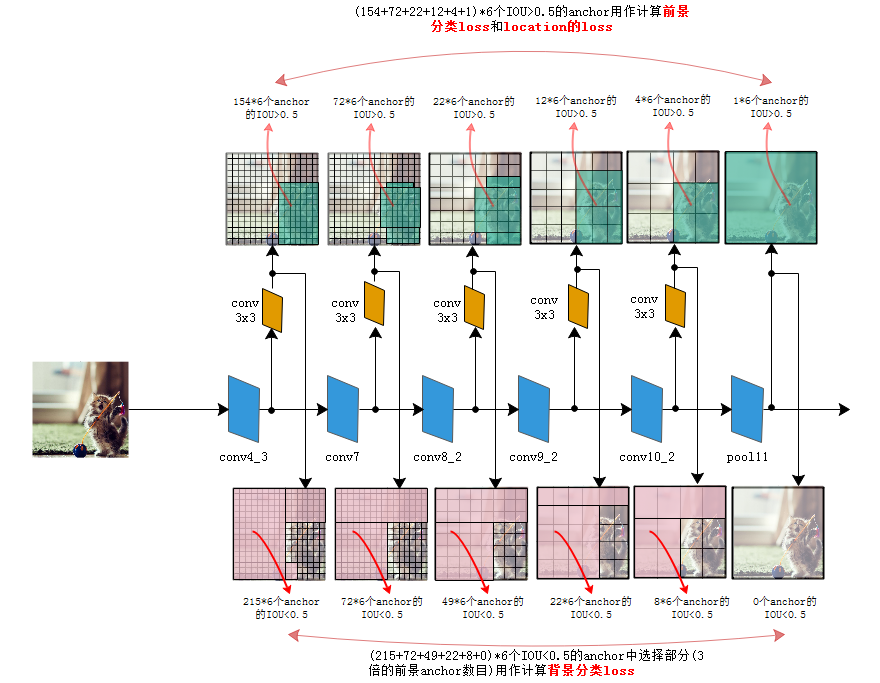
2.2.4.3 SSD在6个层级上进行回归
3 总结
4 SSD的Gluon实现
4.1 类别预测
- 假设物体有
n类,则需要对锚框作n+1个分类,其中类0表示背景。以输入像素为中心输入a个锚框,设高、宽分别为h、w,会有a*h*w个预测结果。 - 使用卷积层的通道来输出类别预测。如果使用全连接层作为输出,可能会导致有过多的模型参数。NIN
类别预测层使用一个保持输入高宽的卷积层,其输出的
(x,y)像素通道里包含了以输入(x,y)像素为中心的所有锚框的类别预测。其输出通道数为a(n+1),其中通道i(n+1)是第 i 个锚框预测的背景置信度,而通道i(n+1)+j+1则是第 i 锚框预测的第 j 类物体的置信度。def cls_predictor(num_anchors, num_classes): return nn.Conv2D(num_anchors * (num_classes + 1), kernel_size=3, padding=1)- 1
- 2
- 3
定义分类器:
指定a和n后,它使用一个填充为 1 的3×3卷积层。注意到我们使用了较小的卷积窗口,它可能不能覆盖锚框定义的区域。所以我们需要保证前面的卷积层能有效的将较大的锚框区域的特征浓缩到一个3×3的窗口里。4.2 边界框预测
对每个锚框我们需要预测如何将其变换到真实的物体边界框。变换由一个长为 4 的向量来描述,分别表示左下和右上的 x、y 轴坐标偏移。与类别预测类似,这里我们同样使用一个保持高宽的卷积层来输出偏移预测,它有 4a 个输出通道,对于第 i 个锚框,它的偏移预测在
4i到4i+3这 4 个通道里。def bbox_predictor(num_anchors): return nn.Conv2D(num_anchors * 4, kernel_size=3, padding=1)- 1
- 2
4.3 合成多层的预测输出
SSD 中会在多个尺度上进行预测。由于每个尺度上的输入高宽和锚框的选取不一样,导致其形状各不相同。下面例子构造两个尺度的输入,其中第二个为第一个的高宽减半。然后构造两个类别预测层,其分别对每个输入像素构造 5 个和 3 个锚框。
def forward(x, block): block.initialize() return block(x) - 假设物体有