Keras LSTM时间序列预测

使用Keras LSTM预测时间序列

参考文章：

Kesci： Keras 实现 LSTM——时间序列预测：https://www.cnblogs.com/mtcnn/p/9411597.html

读取数据

data_path = "/mnt/X500/farmers/tongyao/机器学习项目练习/industry_timeseries/"

#查看其中一个地区的训练数据
import pandas as pd
import numpy as np
from keras.models import Sequential
from keras.layers import Dense, LSTM, Dropout, Flatten
import matplotlib.pyplot as plt
import glob, os
import seaborn as sns
import sys
from sklearn.preprocessing import MinMaxScaler
%matplotlib inline

columns = ['YEAR','MONTH','DAY','TEMP_HIG','TEMP_COL','AVG_TEMP','AVG_WET','DATA_COL']
data = pd.read_csv(data_path + 'timeseries_train_data/2.csv', names=columns)
data.head()

	YEAR	MONTH	DAY	TEMP_HIG	TEMP_COL	AVG_TEMP	AVG_WET	DATA_COL
0	2015	2	1	1.9	-0.4	0.7875	75.000	160.477961
1	2015	2	2	6.2	-3.9	1.7625	77.250	129.268657
2	2015	2	3	7.8	2.0	4.2375	72.750	107.316539
3	2015	2	4	8.5	-1.2	3.0375	65.875	132.549075
4	2015	2	5	7.9	-3.6	1.8625	55.375	91.082841

数据预处理

# 数据预处理：将序列数据转化为监督问题数据
from pandas import DataFrame
from pandas import concat

def series_to_supervised(data, n_in=1, n_out=1, dropnan=True):
    n_vars = 1 if type(data) is list else data.shape[1]
    df = DataFrame(data)
    cols, names = [], []
    # i: n_in, n_in-1, ..., 1
    # 代表t-n_in, ... ,t-1
    for i in range(n_in, 0, -1):
        cols.append(df.shift(i))
        names += [('var%d(t-%d)' % (j+1, i)) for j in range(n_vars)]
    for i in range(0, n_out):
        cols.append(df.shift(-i))
        if i == 0:
            names += [('var%d(t)' % (j+1)) for j in range(n_vars)]
        else:
            names += [('var%d(t+%d)' % (j+1, i)) for j in range(n_vars)]
    agg = concat(cols, axis=1)
    agg.columns = names
    if dropnan:
        agg.dropna(inplace=True)
    return agg

# 将数据归一化到0-1之间,无量纲化
scaler = MinMaxScaler(feature_range=(0,1))
scaled_data = scaler.fit_transform(data[['DATA_COL','TEMP_HIG','TEMP_COL','AVG_TEMP','AVG_WET']].values)

# 将时序数据转换为监督问题数据
reframed = series_to_supervised(scaled_data, 1, 1)

#删除无用的label数据
reframed.drop(reframed.columns[[6,7,8,9]], axis=1, inplace=True)
print(reframed.info())
reframed.head()

运行结果

<class 'pandas.core.frame.DataFrame'>
Int64Index: 577 entries, 1 to 577
Data columns (total 6 columns):
var1(t-1)    577 non-null float64
var2(t-1)    577 non-null float64
var3(t-1)    577 non-null float64
var4(t-1)    577 non-null float64
var5(t-1)    577 non-null float64
var1(t)      577 non-null float64
dtypes: float64(6)
memory usage: 31.6 KB
None

	var1(t-1)	var2(t-1)	var3(t-1)	var4(t-1)	var5(t-1)	var1(t)
1	0.122335	0.049869	0.265823	0.212693	0.599165	0.096338
2	0.096338	0.162730	0.177215	0.236842	0.636743	0.078052
3	0.078052	0.204724	0.326582	0.298142	0.561587	0.099070
4	0.099070	0.223097	0.245570	0.268421	0.446764	0.064529
5	0.064529	0.207349	0.184810	0.239319	0.271399	0.085949

数据划分

# 数据集划分,选取前400天的数据作为训练集,中间150天作为验证集,其余的作为测试集
train_days = 400
valid_days = 150
values = reframed.values
train = values[:train_days, :]
valid = values[train_days:train_days+valid_days, :]
test = values[train_days+valid_days:, :]
train_X, train_y = train[:, :-1], train[:, -1]
valid_X, valid_y = valid[:, :-1], valid[:, -1]
test_X, test_y = test[:, :-1], test[:, -1]

# 将数据集重构为符合LSTM要求的数据格式,即 [样本，时间步，特征]
train_X = train_X.reshape((train_X.shape[0], 1, train_X.shape[1]))
valid_X = valid_X.reshape((valid_X.shape[0], 1, valid_X.shape[1]))
test_X = test_X.reshape((test_X.shape[0], 1, test_X.shape[1]))
print(train_X.shape, train_y.shape, valid_X.shape, valid_y.shape, test_X.shape, test_y.shape)

(400, 1, 5) (400,) (150, 1, 5) (150,) (27, 1, 5) (27,)

训练模型

使用Keras的Sequential搭建模型

model = Sequential()
model.add(LSTM(50, activation='relu',input_shape=(train_X.shape[1], train_X.shape[2]), return_sequences=True))
model.add(Flatten())
model.add(Dense(1, activation='linear'))
model.compile(loss='mean_squared_error', optimizer='adam') 
model.summary()

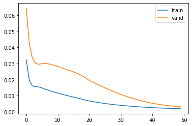
# fit network
hist = model.fit(train_X, train_y, epochs=50, batch_size=32, validation_data=(valid_X, valid_y), verbose=1, shuffle=False)

# plot history
plt.plot(hist.history['loss'], label='train')
plt.plot(hist.history['val_loss'], label='valid')
plt.legend()
plt.show()

输出结果

_________________________________________________________________
Layer (type)                 Output Shape              Param #   
=================================================================
lstm_21 (LSTM)               (None, 1, 50)             11200     
_________________________________________________________________
flatten_3 (Flatten)          (None, 50)                0         
_________________________________________________________________
dense_19 (Dense)             (None, 1)                 51        
=================================================================
Total params: 11,251
Trainable params: 11,251
Non-trainable params: 0
_________________________________________________________________
Train on 400 samples, validate on 150 samples
Epoch 1/50
400/400 [==============================] - 3s 6ms/step - loss: 0.0325 - val_loss: 0.0644
Epoch 2/50
400/400 [==============================] - 0s 152us/step - loss: 0.0196 - val_loss: 0.0425
...
Epoch 50/50
400/400 [==============================] - 0s 176us/step - loss: 0.0019 - val_loss: 0.0031

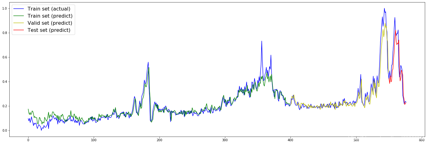
看看预测结果如何

plt.figure(figsize=(24,8))
train_predict = model.predict(train_X)
valid_predict = model.predict(valid_X)
test_predict = model.predict(test_X)
plt.plot(values[:, -1], c='b', label="Train set (actual)")
plt.plot([x for x in train_predict], c='g', label="Train set (predict)")
plt.plot([None for _ in train_predict] + [x for x in valid_predict], c='y', label="Valid set (predict)")
plt.plot([None for _ in train_predict] + [None for _ in valid_predict] + [x for x in test_predict], c='r', label="Test set (predict)")
plt.legend(fontsize=16)
plt.show()

、