使用Keras进行时间序列预测回归问题的LSTM实现

版权声明：本文为博主原创文章，欢迎交流分享，未经博主允许不得转载。 https://blog.csdn.net/HHTNAN/article/details/82462901

基本简介

LSTM_learn
使用Keras进行时间序列预测回归问题的LSTM实现

数据
数据来自互联网，这些数据用于预测航空公司的人数，我们使用LSTM网络来解决这个问题
关于此处模型构建，只对keras部分代码做重点的介绍

模型构建与编译

def build_model():
    # input_dim是输入的train_x的最后一个维度，train_x的维度为(n_samples, time_steps, input_dim)
    model = Sequential()
    #部分注释是对于老版本的kreas,支持，2.2.2不支持
    # model.add(LSTM(input_dim=1, output_dim=50, return_sequences=True))
    #2.2.2 keras
    model.add(LSTM(input_shape=(None, 1), units=100, return_sequences=False))
    #①
    # model.add(LSTM(units=100, return_sequences=False))
    # model.add(Dense(output_dim=1))

    model.add(Dense(units=1))
    model.add(Activation('linear'))

    model.compile(loss='mse', optimizer='rmsprop')
    return model

①上面代码是建立了一个序列模型，采用的lstm,这里面关于参数这里要重点说明，return_sequences=True与False,比如说在我们设置。model.add(LSTM(input_shape=(None, 1), units=100, return_sequences=False))中就不需要执行 model.add(LSTM(units=100, return_sequences=False))，但是在我们执行model.add(LSTM(input_shape=(None, 1), units=100, return_sequences=True))时后面是必须要接， model.add(LSTM(units=100, return_sequences=False))的
具体原因及扩展原因如下：

Understand the Difference Between Return Sequences and Return States for LSTMs in Keras
Kears LSTM API 中给出的两个参数描述

return_sequences：默认 False。在输出序列中，返回单个 hidden state值还是返回全部time step 的 hidden state值。 False 返回单个， true 返回全部。
return_state：默认 False。是否返回除输出之外的最后一个状态。

区别 cell state 和 hidden state

LSTM 的网络结构中，直接根据当前 input 数据，得到的输出称为 hidden state。
还有一种数据是不仅仅依赖于当前输入数据，而是一种伴随整个网络过程中用来记忆，遗忘，选择并最终影响 hidden state 结果的东西，称为 cell state。 cell state 就是实现 long short memory 的关键。

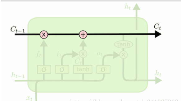
如图所示， C 表示的就是 cell state。h 就是hidden state。（选的图不太好，h的颜色比较浅）。整个绿色的矩形方框就是一个 cell。

cell state 是不输出的，它仅对输出 hidden state 产生影响。

通常情况，我们不需要访问 cell state，除非想设计复杂的网络结构时。例如在设计 encoder-decoder 模型时，我们可能需要对 cell state 的初始值进行设定。

keras 中设置两种参数的讨论

1.return_sequences=False && return_state=False

h = LSTM(X)

Keras API 中，return_sequences和return_state默认就是false。此时只会返回一个hidden state 值。如果input 数据包含多个时间步，则这个hidden state 是最后一个时间步的结果

2.return_sequences=True && return_state=False

LSTM(1, return_sequences=True)

输出的hidden state 包含全部时间步的结果。

3.return_sequences=False && return_state=True

lstm1, state_h, state_c = LSTM(1, return_state=True)

lstm1 和 state_h 结果都是 hidden state。在这种参数设定下，它们俩的值相同。都是最后一个时间步的 hidden state。 state_c 是最后一个时间步 cell state结果。

为什么要保留两个值一样的参数？ 马上看配置4就会明白

为了便于说明问题，我们给配置3和配置4一个模拟的结果，程序结果参考reference文献。

[array([[ 0.10951342]], dtype=float32), # lstm1
 array([[ 0.10951342]], dtype=float32), # state_h
 array([[ 0.24143776]], dtype=float32)] # state_c

3.return_sequences=True && return_state=True

lstm1, state_h, state_c = LSTM(1, return_sequences=True, return_state=True)

此时，我们既要输出全部时间步的 hidden state ，又要输出 cell state。

lstm1 存放的就是全部时间步的 hidden state。

state_h 存放的是最后一个时间步的 hidden state

state_c 存放的是最后一个时间步的 cell state

一个输出例子，假设我们输入的时间步 time step=3

[array([[[-0.02145359],
        [-0.0540871 ],
        [-0.09228823]]], dtype=float32),
 array([[-0.09228823]], dtype=float32),
 array([[-0.19803026]], dtype=float32)]

可以看到state_h 的值和lstm1的最后一个时间步的值相同。

state_c 则表示最后一个时间步的 cell state

Reference
https://machinelearningmastery.com/return-sequences-and-return-states-for-lstms-in-keras/

完整代码：

import pandas as pd
import numpy as np
import matplotlib.pyplot as plt
from sklearn.preprocessing import MinMaxScaler
from keras.models import Sequential
from keras.layers import LSTM, Dense, Activation

def load_data(file_name, sequence_length=10, split=0.8):
    df = pd.read_csv(file_name, sep=',', usecols=[1])

    data_all = np.array(df).astype(float)
    scaler = MinMaxScaler()
    data_all = scaler.fit_transform(data_all)
    data = []
    print("len(data_all)={}".format(len(data_all)))
    for i in range(len(data_all) - sequence_length - 1):
        print("i={}, (i + sequence_length + 1)={}".format(i, i + sequence_length + 1))
        data.append(data_all[i: i + sequence_length + 1])
    reshaped_data = np.array(data).astype('float64')
    np.random.shuffle(reshaped_data)#（133，11，1）
    # 对x进行统一归一化，而y则不归一化
    #行全部取，11列中除了最后一列不取（133，10，1）
    x = reshaped_data[:, :-1]
    #行全部取，11列中只取最后一列（133，1）
    y = reshaped_data[:, -1]
    #分割数
    split_boundary = int(reshaped_data.shape[0] * split)
    train_x = x[: split_boundary]
    test_x = x[split_boundary:]

    train_y = y[: split_boundary]
    test_y = y[split_boundary:]
    print("train_x={}, train_y={}, test_x={}, test_y={}".format(train_x.shape, train_y.shape, test_x.shape, test_y.shape,))
    return train_x, train_y, test_x, test_y, scaler


def build_model():
    # input_dim是输入的train_x的最后一个维度，train_x的维度为(n_samples, time_steps, input_dim)
    model = Sequential()
    # model.add(LSTM(input_dim=1, output_dim=50, return_sequences=True))
    #2.2.2 keras
    model.add(LSTM(input_shape=(None, 1), units=100, return_sequences=False))
    print(model.layers)
    # model.add(LSTM(units=100, return_sequences=False))
    # model.add(Dense(output_dim=1))

    model.add(Dense(units=1))
    model.add(Activation('linear'))

    model.compile(loss='mse', optimizer='rmsprop')
    return model


def train_model(train_x, train_y, test_x, test_y):
    model = build_model()

    try:
        # model.fit(train_x, train_y, batch_size=512, nb_epoch=30, validation_split=0.1)
        model.fit(train_x, train_y, batch_size=512, epochs=30, validation_split=0.1)
        predict = model.predict(test_x)
        predict = np.reshape(predict, (predict.size, ))
    except KeyboardInterrupt:
        print(predict)
        print(test_y)
    print("predict={},test_y={}".format(predict,test_y))
    # print(test_y)
    try:
        fig = plt.figure(1)
        plt.plot(predict, 'r:')
        plt.plot(test_y, 'g-')
        plt.legend(['predict', 'true'])
    except Exception as e:
        print(e)
    return predict, test_y


if __name__ == '__main__':
    train_x, train_y, test_x, test_y, scaler = load_data('international-airline-passengers.csv')
    train_x = np.reshape(train_x, (train_x.shape[0], train_x.shape[1], 1))
    test_x = np.reshape(test_x, (test_x.shape[0], test_x.shape[1], 1))
    print("train_x.shape={},test_x.shape={}".format(train_x.shape,test_x.shape))
    predict_y, test_y = train_model(train_x, train_y, test_x, test_y)
    #返回原来的对应的预测数值
    predict_y = scaler.inverse_transform([[i] for i in predict_y])
    test_y = scaler.inverse_transform(test_y)
    fig2 = plt.figure(2)
    plt.plot(predict_y, 'g:')
    plt.plot(test_y, 'r-')
    plt.show()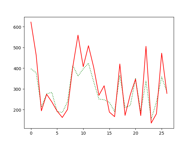

参考文献：
lstm中文网：https://keras.io/layers/recurrent/#lstm
https://blog.csdn.net/yyb19951015/article/details/79740869
https://blog.csdn.net/a819825294/article/details/54376781
https://blog.csdn.net/mebiuw/article/details/52705731
https://blog.csdn.net/hhtnan/article/details/80403146