The probability of an event is a number describing the chance that the event will happen. An event that is certain to happen has a probability of 1. An event that cannot possibly happen has a probability of zero. If there is a chance that an event will happen, then its probability is between zero and 1.
X: event
x: result
If p is a probability, then p/(1 − p) is the corresponding odds;
Then Z= ln(odds) = ln p / (1-p)
e^Z = p/(1-p)
(1-p) e^Z = p
e^Z = (e^Z+1)p
p = e^Z / (1+e^Z) = 1 / (1+e ^(-Z) )
 , This function is called the sigmoid.

At 0 the value of the sigmoid is 0.5. For increasing values of x, the sigmoid will approach 1, and for decreasing values of x, the
sigmoid will approach 0. On a large enough scale (the bottom frame of figure 5.1), the sigmoid looks like a step function.
For the logistic regression classifier we’ll take our features and multiply each one by a weight and then add them up. This result will be put into the sigmoid, and we’ll get a number between 0 and 1. Anything above 0.5 we’ll classify as a 1, and anything below 0.5 we’ll classify as a 0. You can also think of logistic regression as a probability estimate.
The input to the sigmoid function described will be z, where z is given by the following:
![]()
In vector notation we can write this as ![]() , All that means is that we have two vectors of numbers and we’ll multiply each element and add them up to get one number.
, All that means is that we have two vectors of numbers and we’ll multiply each element and add them up to get one number.
Gradient ascent
The first optimization algorithm we’re going to look at is called gradient ascent. Gradient ascent is based on the idea that if we want to find the maximum point on a function, then the best way to move is in the direction of the gradient. We write the gradient ![]() with the symbol and the gradient of a function f(x,y) is given by the equation
with the symbol and the gradient of a function f(x,y) is given by the equation

this gradient means that we’ll move in the x direction by amount![]() and in the y direction by amount
and in the y direction by amount  . The function f(x,y) needs to be defined and differentiable around the points where it’s being evaluated. An example of this is shown in figure 5.2.
The gradient ascent algorithm shown in figure 5.2 takes a step in the direction given by the gradient. The gradient operator will always point in the direction of the greatest increase. We’ve talked about direction, but I didn’t mention anything to do
with magnitude of movement. The magnitude, or step size, we’ll take is given by the parameter ![]() . In vector notation we can write the gradient ascent algorithm as
. In vector notation we can write the gradient ascent algorithm as
![]()

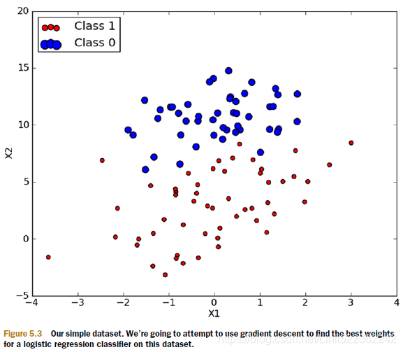
There are 100 data points in figure 5.3. Each point has two numeric features: X1 and X2. We’ll try to use gradient ascent to fit the best parameters for the logistic regression model to our data. We’ll do this by finding the best weights for this given dataset. Pseudocode for the gradient ascent would look like this:
Start with the weights all set to 1
Repeat R number of times:
Calculate the gradient of the entire dataset
Update the weights vector by alpha*gradient
Return the weights vector

# -*- coding: utf-8 -*-
"""
Created on Thu Dec 27 17:37:31 2018
@author: LlQ
"""
import numpy as np
def loadDataSet():
dataMatrixList = [];
labelMatrixList = [];
fileRead = open('testSet.txt')
#in testSet.txt file
# X1 X2 Label
#-0.017612 14.053064 0
#-1.395634 4.662541 1
#-0.752157 6.538620 0
#-1.322371 7.152853 0
#0.423363 11.054677 0
#0.406704 7.067335 1
#...
for line in fileRead.readlines():
lineArray = line.strip().split()
dataMatrixList.append([1.0, float(lineArray[0]), float(lineArray[1])])
labelMatrixList.append(int(lineArray[2]))
return dataMatrixList, labelMatrixList
def sigmoid(intZ):
return 1.0/(1+np.exp(-intZ))
#for R programming, glm will give your the coefficients value
#dataMat--features:
#X0 X1 X2
#1 -0.017612 14.053064
#1 -1.395634 4.662541
#1 ...
#classlabels---x: ([0, 1, ...])
def gradientAscent(dataMatrixList, classLabelList):
#dataMatrix([[1, X1, X2],[1, X1,X2]...])
dataMatrix=np.mat(dataMatrixList)# convert to NumPy matrices
labelMatrix=np.mat(classLabelList).transpose()#100columns-to-100rows
# LabelMatrix([
# 0,
# 1,
# 0,
# 0,
# 0,
# 1,
# ...
# ])
rows, columns = np.shape(dataMatrix) # rows=100, columns=3
alpha = 0.001
maxCycles = 500
weights = np.ones((columns,1))#the best coefficients w: n-rows and 1 column
# ones since sigmoid(x1) or sigmoid(x2)
#weight 3x1
#weights([
# 1,
# 1,
# 1
#])
#print(type(weights)) #ndarray########
for k in range(maxCycles):
#intZ = x * wT #we have two vectors of numbers and we’ll multiply
#each element and add them up to get one number.
#x: feature
#wT: coefficients
#intx = x*bi
#Z = x0 * w0 + x1 * w1 + x2 * w2 + ... + xn * wn
intZ=dataMatrix*weights #matrix
#is not one multiplication but actually 100x3 * 3x1#matrices mulplication
#print(len(intZ)) #100 rows
# print(intZ)
#print("**********************")
sig = sigmoid(intZ)
#print(len(sig)) #100
#print(sig) #0<sig<1
error = (labelMatrix-sig)#matrix
#weights + alpha * (3x100 * 100x1) #matrices mulplication
weights = weights + alpha * dataMatrix.transpose()*error
return weights #matrix 100x1 ########
#dataMatrix 3x100 * vertical List-3x1 matrix
def plotBestFit(coefficientList):
import matplotlib.pyplot as plt
import numpy as np
weights = coefficientList
dataArrList, labelList = loadDataSet()
dataArrList = np.array(dataArrList)
columns = np.shape(dataArrList)[0] #100 row
xcord1 = []; ycord1 = []
xcord2 = []; ycord2 = []
for i in range(columns):
if int(labelList[i]) == 1:
xcord1.append(dataArrList[i,1]) #X1
ycord1.append(dataArrList[i,2]) #X2
else:
xcord2.append(dataArrList[i,1]) #X1
ycord2.append(dataArrList[i,2]) #x2
fig=plt.figure()
ax = fig.add_subplot(111)
ax.scatter(xcord1, ycord1, s=30, c='red', marker='s')
ax.scatter(xcord2, ycord2, s=30, c='green')
x=np.arange(-3.0, 3.0, 0.1)
y=(-weights[0]-weights[1]*x) / weights[2] #y=-(b0+b1x)/b3
ax.plot(x,y) #plot best-fit line
plt.xlabel('X1')
plt.ylabel('X2')
plt.show()
###############################################################################
# import logisticRegression
# from imp import reload
# reload(logisticRegression)
# dataArrList, labelList = logisticRegression.loadDataSet()
# coefficient = logisticRegression.gradientAscent(dataArrList, labelList)
# coefficient
# output:
# matrix([[ 4.12414349],
# [ 0.48007329],
# [-0.6168482 ]])
# logisticRegression.plotBestFit(coefficient.getA())
###############################################################################
def stochasticGradientAscent0(dataMatrixArray, classLabelList):
rows, columns = np.shape(dataMatrixArray)
alpha = 0.01
weightList=np.ones(columns)
for i in range(rows):
sig = sigmoid(sum(dataMatrixArray[i]*weightList)) #float64
error = classLabelList[i] - sig
weightList=weightList + alpha * error * dataMatrixArray[i]
#print(type(weightList)) #ndarray
return weightList
###############################################################################
# import logisticRegression
# from imp import reload
# reload(logisticRegression)
# from numpy import *
# dataArrList, labelList = logisticRegression.loadDataSet()
# coefficientList = logisticRegression.stochasticGradientAscent0(array(dataArrList), labelList)
###############################################################################
def stochasticGradientAscent1(dataMatrixArray, classLabelList, numIter=150):
rows, columns = np.shape(dataMatrixArray)
#alpha=0.01
weightList = np.ones(columns)
for j in range(numIter):
dataIndex = list(range(rows))
for i in range(rows):
#This will improve the oscillations that occur in the dataset
#Alpha decreases as the number of iterations increases,
#but it never reaches 0 because there’s a constant term(0.0001).
#You need to do this so that after a large number of cycles,
#new data still has some impact.
#Perhaps you’re dealing with something that’s changing with time.
#Then you may want to let the constant term(>0.0001) be larger
#to give more weight to new values.
#The second thing about the decreasing alpha function is that
#it decreases by 1/(j+i); j is the index of the number of times
#you go through the dataset,
#and i is the index of the example in the training set.
#This gives an alpha that isn’t strictly decreasing when j<<max(i).
#The avoidance of a strictly decreasing weight is shown to
#work in other optimization algorithms, such as simulated annealing.
alpha = 4/(1.0+j+i)+0.0001 #alpha changes on each iteration.
#you’re randomly selecting each instance to use in updating the
#weights. This will reduce the periodic variations
randIndex = int(np.random.uniform(0,len(dataIndex)))
sig = sigmoid(sum(dataMatrixArray[randIndex]*weightList))
error = classLabelList[randIndex] - sig
weightList = weightList + alpha*error*dataMatrixArray[randIndex]
del(dataIndex[randIndex])
return weightList
#Coefficient convergence in stocGradAscent1() with random vector selection and
#decreasing alpha. This method is much faster to converge than using a fixed alpha
#dealing with missing values in the data
#Use the feature’s mean value from all the available data.
#■ Fill in the unknown with a special value like -1.
#■ Ignore the instance.
#■ Use a mean value from similar items.
#■ Use another machine learning algorithm to predict the value.
#replace all the unknown values with a real number(0) because we’re using NumPy
#in NumPy arrays can’t contain a missing value
#we want a value(0) that won’t impact the weight(coefficient) during the update
#The weights are updated according to
# weights = weights + alpha * error * dataMatrix[randIndex]
#1) If dataMatrix is 0 for any feature, then the weight for that feature will
# simply be weights = weights
#2) the error term will not be impacted by this because sigmoid(0)=0.5,
# which is totally neutral for predicting the class.
#3) none of the features take on 0 in the data, so in some sense
# it’s a special value.
#Second, there was a missing class label in the test data. I simply threw it
#out. It’s hard to replace a missing class label. This solution makes sense
#given that we’re using logistic regression, but it may not make sense with
#something like kNN(prediction).
###############################################################################
# import logisticRegression
# import numpy as np
# from imp import reload
# reload(logisticRegression)
# dataArrList, labelList = logisticRegression.loadDataSet()
# coefficientList = logisticRegression.stochasticGradientAscent0(np.array(dataArrList), labelList)
# logisticRegression.plotBestFit(coefficientList)
###############################################################################
#This takes the weights and an input vector and calculates the sigmoid.
#If the value of the sigmoid is more than 0.5,
#it’s considered a 1; otherwise, it’s a 0
def classifyVector(inXArray, weightList):
prob = sigmoid(sum(inXArray*weightList))
if prob > 0.5:
return 1.0
else:
return 0.0
def colicTest():
frTrain = open('horseColicTraining.txt')
frTest = open('horseColicTest.txt')
trainingSet =[]
trainingLabels=[]
for line in frTrain.readlines():
currentLine = line.strip().split('\t')
lineArray = []
for i in range(21):
lineArray.append(float(currentLine[i]))
trainingSet.append(lineArray)
trainingLabels.append(float(currentLine[21]))
#coefficients
trainWeights = stochasticGradientAscent1(np.array(trainingSet), trainingLabels, 500)
errorCount=0
numTestVec = 0.0
for line in frTest.readlines():
numTestVec += 1.0
currentLine=line.strip().split('\t')
lineArray=[]
for i in range(21):
lineArray.append(float(currentLine[i]))
if int(classifyVector(np.array(lineArray), trainWeights)) != \
int(currentLine[21]):
errorCount +=1
errorRate = (float(errorCount)/numTestVec)
print ("the error rate of this test is: %f" % errorRate)
return errorRate
def multiTest():
numTests = 10;
errorSum = 0.0
for k in range(numTests):
errorSum += colicTest()
print("after %d iterations the average error rate is: %f" % (numTests, \
errorSum/float(numTests)))
#This wasn’t bad with over 30% of the values missing. You can alter the number
#of iterations in colicTest() and the alpha size(0.01 to 0.0001, the constant item)
# in stochGradAscent1() to get results approaching a 20% error rate.
###############################################################################
# import logisticRegression
# import numpy as np
# from imp import reload
# reload(logisticRegression)
# logisticRegression.multiTest()
# output:
# the error rate of this test is: 0.253731
# the error rate of this test is: 0.373134
# the error rate of this test is: 0.373134
# the error rate of this test is: 0.402985
# the error rate of this test is: 0.388060
# the error rate of this test is: 0.417910
# the error rate of this test is: 0.417910
# the error rate of this test is: 0.283582
# the error rate of this test is: 0.328358
# the error rate of this test is: 0.358209
# after 10 iterations the average error rate is: 0.359701
# # logisticRegression.multiTest()
# output:
# the error rate of this test is: 0.358209
# the error rate of this test is: 0.417910
# the error rate of this test is: 0.358209
# the error rate of this test is: 0.253731
# the error rate of this test is: 0.298507
# the error rate of this test is: 0.388060
# the error rate of this test is: 0.373134
# the error rate of this test is: 0.313433
# the error rate of this test is: 0.313433
# the error rate of this test is: 0.328358
# after 10 iterations the average error rate is: 0.340299
###############################################################################

