conv2d(
    input,
    filter,
    strides,
    padding,
    use_cudnn_on_gpu=None,
    data_format=None,
    name=None
)input是一个4d输入[batch_size,in_height,in_width,n_channels],表示图片的批数,大小和通道。filter是一个4d输入[filter_height,filter_width,in_channels,out_channels],表示kernel的大小,输入通道数和输出通道数,其中输出通道数表示从上一层提取多少特征。strides是一个1d输入,长度为4,其中stride[0]和stride[3]必须为1,一般格式为[1, stride[1], stride[2], 1],在大部分情况下,因为在height和width上的步进设为一样,因此通常为[1, stride, stride, 1]。
计算公式为:
output[b,i,j,k]=∑di,dj,qinput[b,strides[1]∗i+di,strides[2]∗j+dj,q]∗filter[di,dj,q,k]
其中b为batch_id, i,j分别是图片的像素索引, k是输出通道的索引,q是输入通道的索引,从公式可以看出,conv2d是将一个图片的所有输入通道卷积合成一个输出通道的,这个和tf.nn.depthwise_conv2d有所不同。padding是一个字符串输入,分为SAME和VALID分别表示是否需要填充,因为卷积完之后因为周围的像素没有卷积到,因此一般是会出现卷积完的输出尺寸小于输入的现象的,这时候可以利用填充如:
Figure1, No padding, not strides
Figure2, Half padding, not strides
Figure3, No padding, stride 2
Figure4, padding and stride 2
例子:
import tensorflow as tf
input_data = tf.Variable( np.random.rand(2,4,4,2), dtype = np.float32 )
filter_data = tf.Variable( np.random.rand(4, 4, 2, 3), dtype = np.float32)
y = tf.nn.conv2d(input_data, filter_data, strides = [1, 1, 1, 1], padding = 'SAME')
with tf.Session() as sess:
    sess.run(tf.global_variables_initializer())
    print(sess.run(y))
输出
[[[[ 3.02819729  4.65413046  4.60143995]
   [ 3.97926784  5.43468952  5.70441341]
   [ 1.99813139  3.84203005  4.01785088]
   [ 1.76864231  2.11749601  2.94542313]]

  [[ 4.17383385  6.33559418  5.85187054]
   [ 6.31012106  8.01992798  7.54992771]
   [ 5.45781803  5.69342327  5.68077469]
   [ 2.72828531  2.51591063  3.32510877]]

  [[ 3.64953375  4.43592453  4.09911633]
   [ 4.65612841  6.32581902  6.22575855]
   [ 4.33319664  4.41670799  5.05007505]
   [ 2.71822929  1.97995758  2.72764444]]

  [[ 1.73219407  2.33855247  3.12495542]
   [ 3.69550705  3.35003376  2.54378915]
   [ 2.04344559  1.80226278  2.64786339]
   [ 1.94504452  1.59554958  1.87581062]]]


 [[[ 3.4564662   5.85969734  4.95160866]
   [ 4.06665373  7.86626101  7.41516113]
   [ 4.18327904  6.12413883  6.04700041]
   [ 3.60840511  3.35275459  4.22719717]]

  [[ 5.73996019  7.98878765  6.5777669 ]
   [ 8.04671001  9.05361843  8.77891731]
   [ 6.95388889  6.94798946  7.95665741]
   [ 4.04243183  4.85149479  6.03445339]]

  [[ 3.30251527  4.77820301  5.22986221]
   [ 4.99443626  7.29389048  6.09803677]
   [ 4.35838127  4.46987915  5.35628796]
   [ 3.32821941  2.85371852  3.90200329]]

  [[ 3.1087513   3.78305531  2.81782913]
   [ 4.51704264  3.92821026  3.95264912]
   [ 3.55470753  2.33432341  3.7320199 ]
   [ 2.91192126  1.69659698  1.93430305]]]]
我们该如何看待这种数据呢,如何将其和图片像素对应起来呢?
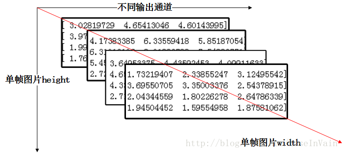
以上就是输出的第一个batch的可视化,多个batch叠加即可。