【R描述统计分析】数据的分布

分布函数

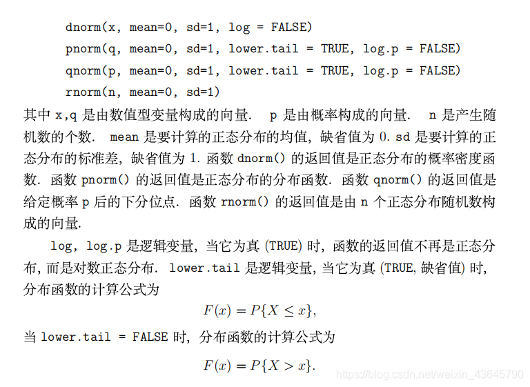
正态分布

dnorm 概率密度函数f(x)，或分布律pk
pnorm 分布函数F(x)
qnorm 分布函数的反函数F-1§， 即给定概率p后，求其下分位点
rnorm 产生随机数

r<-rnorm(100,0,1)
dnorm(x,mean=0,sd=1)
pnorm(q,mean=0,sd=1)
qnorm(p,mean=0,sd=1)
rnorm(n,mean=0,sd=1)

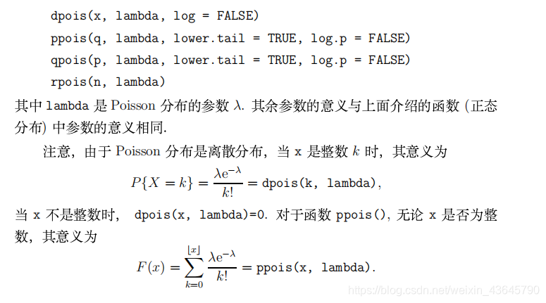
Possion分布

dpois(x,lambda)
ppois(q,lambda)
qpois(p,lambda)
rpois(n,lambda)

其他分布函数或分布律

分布	R软件中的名称	附加参数
binomial	binom	size, prob
Cauchy	cauchy	location scale
chi-squared	chisq	df, ncp
exponential	exp	rate
F	f	df1,df2,ncp
geometric	geom	prob
hypergeometric	hyper	m,n,k
log-normal	lnorm	meanlog,sdlog
logistic	logis	location,scale
normal	norm	mean,sd
Possion	pois	lambda
Student’s t	t	df,ncp
uniform	unif	min,max
Weibull	weibull	shape,scale
beta	beta	shape1,shape2,ncp

图形

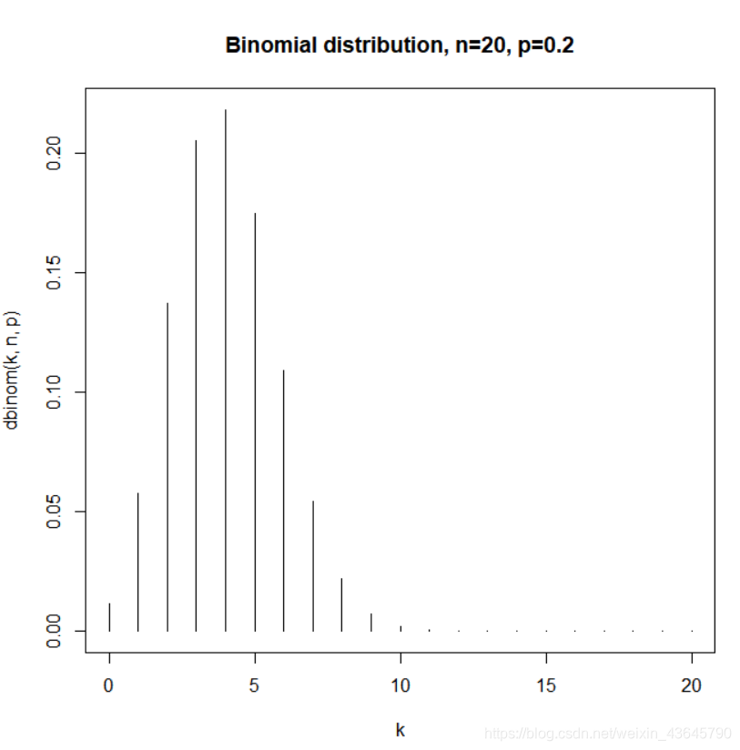
二项分布

n<-20
p<-0.2
k<-seq(0,n)
plot(k,dbinom(k,n,p),type='h',main='Binomial distribution, n=20, p=0.2',xlab='k')

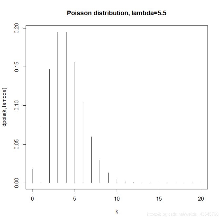
泊松分布

lambda<-4.0
k<-seq(0,20)
plot(k,dpois(k,lambda),type='h',main='Poisson distribution, lambda=5.5',xlab='k')

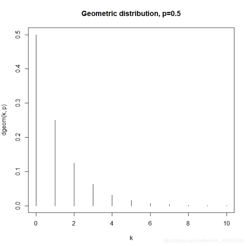
几何分布

p<-0.5
k<-seq(0,10)
plot(k,dgeom(k,p),type='h',main='Geometric distribution, p=0.5',xlab='k')

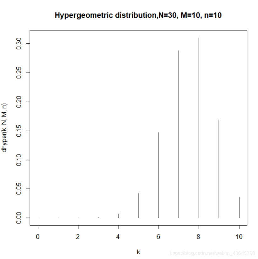
超几何分布

N<-30
M<-10
n<-10
k<-seq(0,10)
plot(k,dhyper(k,N,M,n),type='h',main='Hypergeometric distribution,N=30, M=10, n=10',xlab='k')

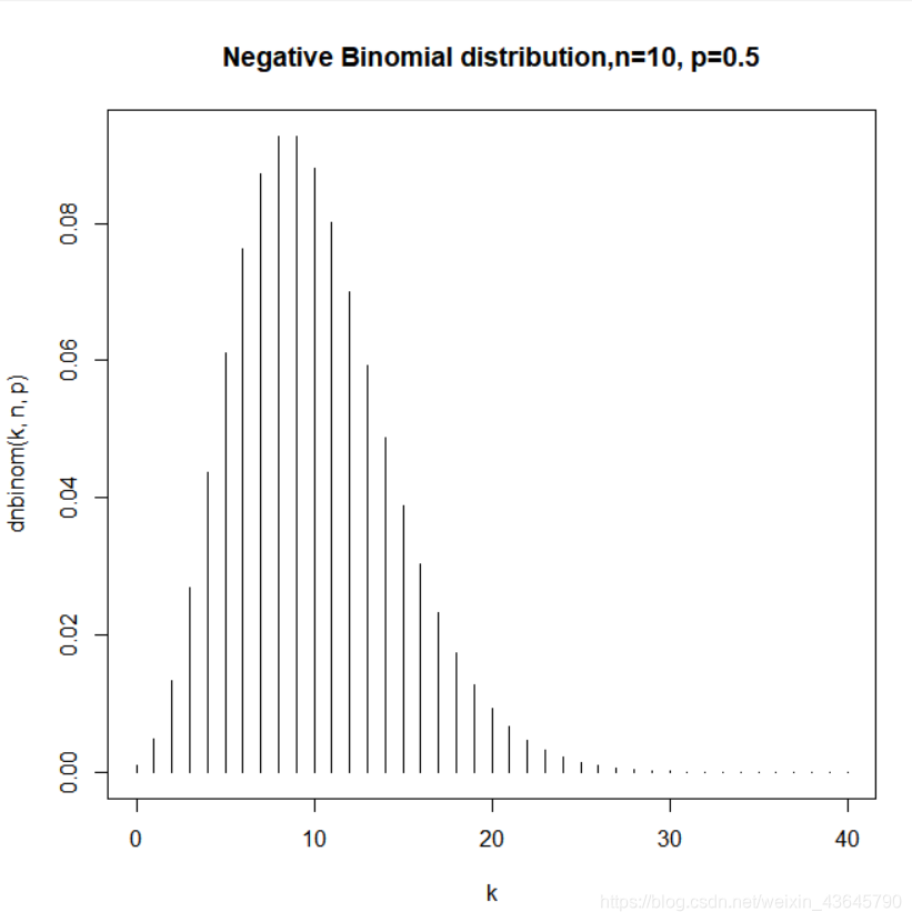
负二项分布

n<-10
p<-0.5
k<-seq(0,40)
plot(k, dnbinom(k,n,p), type='h',main='Negative Binomial distribution,n=10, p=0.5',xlab='k')

分布图

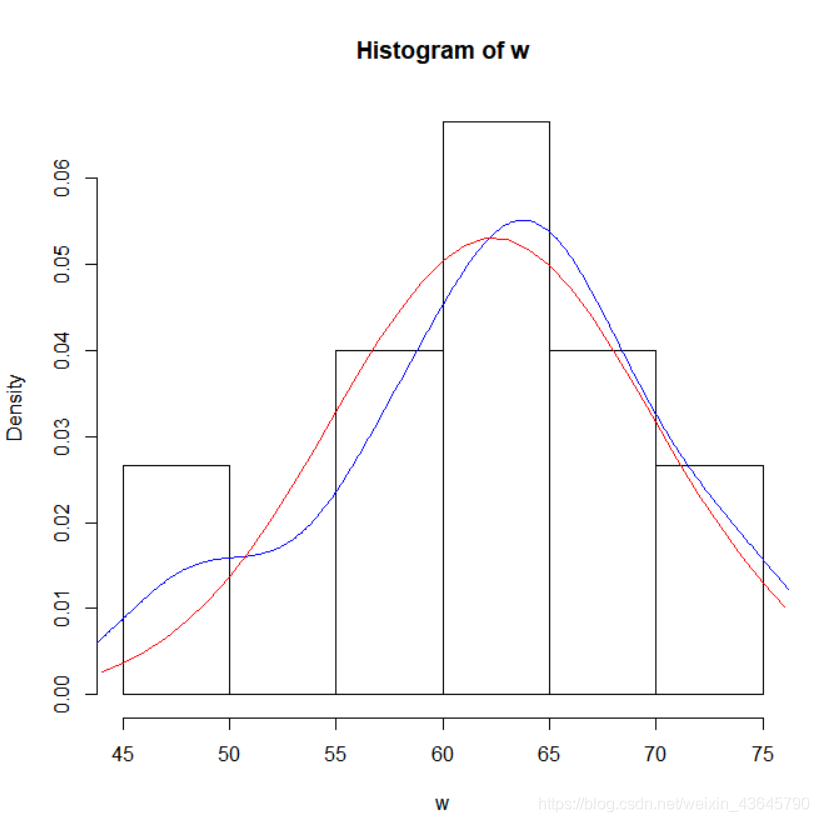
直方图与核密度估计函数

学生体重的直方图和核密度估计图，并与正态分布的概率密度函数相对比

w <- c(75.0, 64.0, 47.4, 66.9, 62.2, 62.2, 58.7, 63.5, 66.6, 64.0, 57.0, 69.0, 56.9, 50.0, 72.0)
hist(w, freq=FALSE)
lines(density(w),col="blue")
x<-44:76
lines(x, dnorm(x, mean(w), sd(w)), col="red")

得到的结果如图：

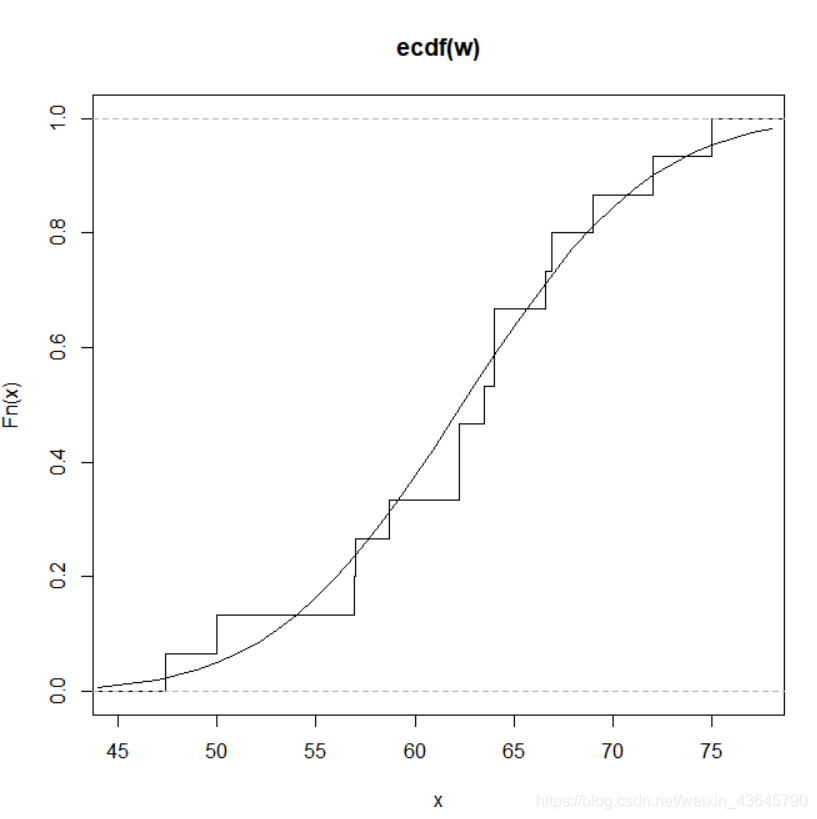
经验分布

经验分布图和相应的正态分布图

w <- c(75.0, 64.0, 47.4, 66.9, 62.2, 62.2, 58.7, 63.5, 66.6, 64.0, 57.0, 69.0, 56.9, 50.0, 72.0)
plot(ecdf(w),verticals = TRUE, do.p = FALSE)
x<-44:78
lines(x, pnorm(x, mean(w), sd(w)))

正态QQ图

w <- c(75.0, 64.0, 47.4, 66.9, 62.2, 62.2, 58.7, 63.5, 66.6, 64.0, 57.0, 69.0, 56.9, 50.0, 72.0)
qqnorm(w); qqline(w)

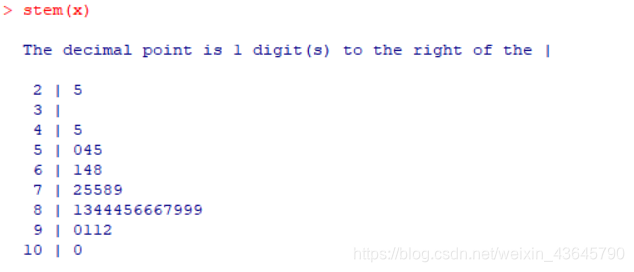
茎叶图

x<-c(25, 45, 50, 54, 55, 61, 64, 68, 72, 75, 75, 
     78, 79, 81, 83, 84, 84, 84, 85, 86, 86, 86, 
     87, 89, 89, 89, 90, 91, 91, 92, 100)
stem(x) 

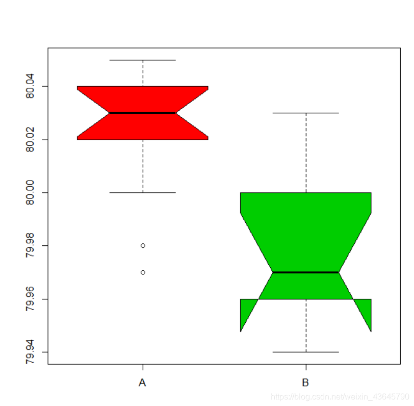
箱线图

两种方法得到的数据

A <- c(79.98, 80.04, 80.02, 80.04, 80.03, 80.03, 80.04,
       79.97, 80.05, 80.03, 80.02, 80.00, 80.02)    
B <- c(80.02, 79.94, 79.98, 79.97, 79.97, 80.03, 79.95, 79.97)        
boxplot(A, B, notch=T, names=c('A', 'B'), col=c(2,3))

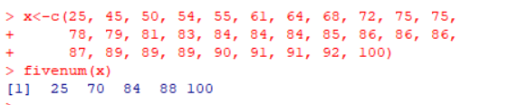
五数总括

x<-c(25, 45, 50, 54, 55, 61, 64, 68, 72, 75, 75, 
     78, 79, 81, 83, 84, 84, 84, 85, 86, 86, 86, 
     87, 89, 89, 89, 90, 91, 91, 92, 100)
fivenum(x)