【放假第2天】人工智能-逻辑回归多分类-代码

1.简单逻辑回归

import numpy as np
import matplotlib.pyplot as plt
from sklearn.preprocessing import PolynomialFeatures
from sklearn.linear_model import LinearRegression

m=100
x=6*np.random.rand(m,1)-3
y=0.5*x**2+x+2+np.random.randn(m,1)


plt.plot(x,y,'b')
plt.show()

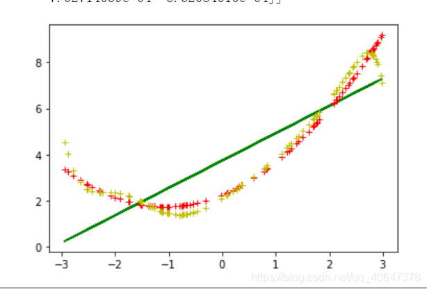
结果…还是画散点图吧
在这里插入图片描述

#不同的指数的回归
.fit_transform:
https://blog.csdn.net/weixin_38278334/article/details/82971752

import numpy as np
import matplotlib.pyplot as plt
from sklearn.preprocessing import PolynomialFeatures
from sklearn.linear_model import LinearRegression

m=100
x=6*np.random.rand(m,1)-3
y=0.5*x**2+x+2+np.random.randn(m,1)

#plt.plot(x,y,'b')

d={1:'g-',2:'r+',10:'y+'}
#这个是一个字典  上面是颜色
for i in d:
    poly_features=PolynomialFeatures(degree=i,include_bias=False)
    x_poly=poly_features.fit_transform(x)
    #这个是preprocessing带的功能 i是几阶 它会存为 x x^2 x^3   后面是不包括w0  只有有x0时候才有w0 有x0是intercept为true
    #改：include_bias=True下面lin_reg=LinearRegression(fit_intercept=True)
    #打印看一下数据特征
    print(x[0])
    print(x_poly[0])
    print(x_poly[:,0])
    lin_reg=LinearRegression()
    lin_reg.fit(x_poly,y)
    print(lin_reg.intercept_,lin_reg.coef_)
    
    y_predict=lin_reg.predict(x_poly)
    plt.plot(x_poly[:,0],y_predict,d[i])

plt.show()

结果：
在这里插入图片描述

#保险公司数据

import pandas as pd
#import numpy as np
import matplotlib.pyplot as plt
from sklearn.preprocessing import PolynomialFeatures
from sklearn.linear_model import LinearRegression

data=pd.read_csv('./insurance.csv')
print(type(data))
print(data.head())
print(data.tail())
#describe做简单的统计摘要，均值，标准差那种
print(data.describe())

#采样要均匀  想要模型来一个就准确，在训练的时候就给他练了，比较平均，10-20岁-->60岁die
data_count=data['age'].value_counts()
print(data_count)
#data_count[:10].plt(kind='bar')
plt.show()
plt.savefig('./temp')
#上面只是为了展示基础知识

#看相关性
print(data.corr())


reg=LinearRegression()
#x=data["age","sex","bmi","children","smoker","region"]   要注意细节呀亲爱的
x = data[['age', 'sex', 'bmi', 'children', 'smoker', 'region']]
y=data["charges"]
#不能转换 string to float  之前遇到的那个报错啊！！ 上面是为了人为操作，不能指望它们

#填补空缺值，字符转为数字
#https://www.cnblogs.com/BoyceYang/p/8213784.html
x=x.apply(pd.to_numeric,errors='coerce')
y=y.apply(pd.to_numeric,errors='coerce')
x.fillna(0,inplace=True)
y.fillna(0,inplace=True)
# print(x)
# print(y)
#上面是看一看数据类型

#poly_features=PolynomialFeatures(degree=3,indlude_bias=False)  错了一个单词啊
poly_features = PolynomialFeatures(degree=3, include_bias=False)
x_poly=poly_features.fit_transform(x)
reg.fit(x_poly,y)
print(reg.intercept_)
print(reg.coef_)

y_predict=reg.predict(x_poly)
plt.plot(x['age'],y,'b.')
plt.plot(x_poly[:,0],y_predict,'r.')
plt.show()

结果：

在这里插入图片描述

#逻辑回归 sklearn处理鸢尾花数据集

gridSearchCV 自动调参
https://blog.csdn.net/weixin_41988628/article/details/83098130

import numpy as np
from sklearn import datasets
from sklearn.linear_model import LogisticRegression
from sklearn.model_selection import GridSearchCV
#import matplotlib as plt
import matplotlib.pyplot as plt
from time import time

iris=datasets.load_iris()
print(list(iris.keys()))
#数据库里面这个就是三种花,共150条数据，4个属性
print(iris['DESCR'])#通过key从字典里取值
print(iris['feature_names'])

x=iris['data'][:,3:]  #这里去了petal width 花瓣的宽度这个维度 其实是上面看出了这个跟预测的相关性最高
#print(x)

print(iris['target'])
y=iris['target']
#y=(iris['target']==2).astype(np.int)
#Numpy中ndim、shape、dtype、astype的用法 https://blog.csdn.net/Da_wan/article/details/80518725
print(y)

start=time()
param_grid={"tol":[1e-4,1e-3,1e-2],
           "c":[0.4,0.6,0.8]}

#参数参考：https://blog.csdn.net/qq_37007384/article/details/88410998

log_reg=LogisticRegression(multi_class='ovr',solver='sag')
#参数参考：https://blog.csdn.net/qq_27972567/article/details/81949023

log_reg.fit(x, y)

grid_search=GridSearchCV(log_reg,param_grid=param_grid,cv=3)
#参数参考：https://blog.csdn.net/Kyrie_Irving/article/details/90023615

#https://blog.csdn.net/weixin_40283816/article/details/83346098
#print("GridSearchCV took %.2f seconds for %d candidate parameter sttings."%(time()-start,len(grid_result.cv_results_['params'])))
#report(grid_result.cv_results_)


#create a new dataset to predict the result
#参数参考  https://blog.csdn.net/weixin_40103118/article/details/78787454
#numpy.reshape(a,(-1,1))：#将a重新塑形为一列，行数由Numpy根据剩下的维度计算所得。
x_new=np.linspace(0,3,1000).reshape(-1,1)#是在这个区间里生成1000个数
#print(x_new)


# 返回预测属于某标签的概率  https://blog.csdn.net/m0_37870649/article/details/79549142

#NotFittedError: Call fit before prediction   之前报的错，因为 .predict  之前要.fit  log_reg.fit(x, y)意思说它没有训练

y_proba=log_reg.predict_proba(x_new)
y_hat=log_reg.predict(x_new)
print(y_proba)
print(y_hat)

plt.plot(x_new,y_proba[:,2],'g-',label='Iris-Virginica')
plt.plot(x_new, y_proba[:, 1], 'r-', label='Iris-Versicolour')
plt.plot(x_new, y_proba[:, 0], 'b--', label='Iris-Setosa')
plt.show()


print(log_reg.predict([[1.7], [1.5]]))

结果：

[‘data’, ‘target’, ‘target_names’, ‘DESCR’, ‘feature_names’, ‘filename’]
… _iris_dataset:

Iris plants dataset

Data Set Characteristics:

:Number of Instances: 150 (50 in each of three classes)
:Number of Attributes: 4 numeric, predictive attributes and the class
:Attribute Information:
    - sepal length in cm
    - sepal width in cm
    - petal length in cm
    - petal width in cm
    - class:
            - Iris-Setosa
            - Iris-Versicolour
            - Iris-Virginica
            
:Summary Statistics:

============== ==== ==== ======= ===== ====================
                Min  Max   Mean    SD   Class Correlation
============== ==== ==== ======= ===== ====================
sepal length:   4.3  7.9   5.84   0.83    0.7826
sepal width:    2.0  4.4   3.05   0.43   -0.4194
petal length:   1.0  6.9   3.76   1.76    0.9490  (high!)
petal width:    0.1  2.5   1.20   0.76    0.9565  (high!)
============== ==== ==== ======= ===== ====================

[‘sepal length (cm)’, ‘sepal width (cm)’, ‘petal length (cm)’, ‘petal width (cm)’]

[0 0 0 0 0 0 0 0 0 0 0 0 0 0 0 0 0 0 0 0 0 0 0 0 0 0 0 0 0 0 0 0 0 0 0 0 0
0 0 0 0 0 0 0 0 0 0 0 0 0 1 1 1 1 1 1 1 1 1 1 1 1 1 1 1 1 1 1 1 1 1 1 1 1
1 1 1 1 1 1 1 1 1 1 1 1 1 1 1 1 1 1 1 1 1 1 1 1 1 1 2 2 2 2 2 2 2 2 2 2 2
2 2 2 2 2 2 2 2 2 2 2 2 2 2 2 2 2 2 2 2 2 2 2 2 2 2 2 2 2 2 2 2 2 2 2 2 2
2 2]
[0 0 0 0 0 0 0 0 0 0 0 0 0 0 0 0 0 0 0 0 0 0 0 0 0 0 0 0 0 0 0 0 0 0 0 0 0
0 0 0 0 0 0 0 0 0 0 0 0 0 1 1 1 1 1 1 1 1 1 1 1 1 1 1 1 1 1 1 1 1 1 1 1 1
1 1 1 1 1 1 1 1 1 1 1 1 1 1 1 1 1 1 1 1 1 1 1 1 1 1 2 2 2 2 2 2 2 2 2 2 2
2 2 2 2 2 2 2 2 2 2 2 2 2 2 2 2 2 2 2 2 2 2 2 2 2 2 2 2 2 2 2 2 2 2 2 2 2
2 2]

#这个是预测的概率三列是属于不同类别的概率
这个是y=1/(1+e^(-z))的概率
[[7.92387200e-01 2.06999715e-01 6.13085232e-04]
[7.92192982e-01 2.07185792e-01 6.21225735e-04]
[7.91997637e-01 2.07372886e-01 6.29476933e-04]
…
[2.64033781e-05 3.18730603e-01 6.81242993e-01]
[2.60411756e-05 3.18832233e-01 6.81141726e-01]
[2.56839510e-05 3.18933941e-01 6.81040375e-01]]
#下面是哪个类别
[0 0 0 0 0 0 0 0 0 0 0 0 0 0 0 0 0 0 0 0 0 0 0 0 0 0 0 0 0 0 0 0 0 0 0 0 0
0 0 0 0 0 0 0 0 0 0 0 0 0 0 0 0 0 0 0 0 0 0 0 0 0 0 0 0 0 0 0 0 0 0 0 0 0
0 0 0 0 0 0 0 0 0 0 0 0 0 0 0 0 0 0 0 0 0 0 0 0 0 0 0 0 0 0 0 0 0 0 0 0 0
0 0 0 0 0 0 0 0 0 0 0 0 0 0 0 0 0 0 0 0 0 0 0 0 0 0 0 0 0 0 0 0 0 0 0 0 0
0 0 0 0 0 0 0 0 0 0 0 0 0 0 0 0 0 0 0 0 0 0 0 0 0 0 0 0 0 0 0 0 0 0 0 0 0
0 0 0 0 0 0 0 0 0 0 0 0 0 0 0 0 0 0 0 0 0 0 0 0 0 0 0 0 0 0 0 0 0 0 0 0 0
0 0 0 0 0 0 0 0 0 0 0 0 0 0 0 0 0 0 0 0 0 0 0 0 0 0 0 0 0 0 0 0 0 0 0 0 0
0 0 0 0 0 0 0 0 0 0 0 0 0 0 0 0 0 0 0 0 0 0 0 0 0 0 0 0 0 0 0 0 0 0 0 0 0
0 0 0 0 0 0 0 0 0 0 0 0 0 0 1 1 1 1 1 1 1 1 1 1 1 1 1 1 1 1 1 1 1 1 1 1 1
1 1 1 1 1 1 1 1 1 1 1 1 1 1 1 1 1 1 1 1 1 1 1 1 1 1 1 1 1 1 1 1 1 1 1 1 1
1 1 1 1 1 1 1 1 1 1 1 1 1 1 1 1 1 1 1 1 1 1 1 1 1 1 1 1 1 1 1 1 1 1 1 1 1
1 1 1 1 1 1 1 1 1 1 1 1 1 1 1 1 1 1 1 1 1 1 1 1 1 1 1 1 1 1 1 1 1 1 1 1 1
1 1 1 1 1 1 1 1 1 1 1 1 1 1 1 1 1 1 1 1 1 1 1 1 1 1 1 1 1 1 1 1 1 1 1 1 1
1 1 1 1 1 1 1 1 1 1 1 1 1 1 1 1 1 1 1 1 1 1 1 1 1 1 2 2 2 2 2 2 2 2 2 2 2
2 2 2 2 2 2 2 2 2 2 2 2 2 2 2 2 2 2 2 2 2 2 2 2 2 2 2 2 2 2 2 2 2 2 2 2 2
2 2 2 2 2 2 2 2 2 2 2 2 2 2 2 2 2 2 2 2 2 2 2 2 2 2 2 2 2 2 2 2 2 2 2 2 2
2 2 2 2 2 2 2 2 2 2 2 2 2 2 2 2 2 2 2 2 2 2 2 2 2 2 2 2 2 2 2 2 2 2 2 2 2
2 2 2 2 2 2 2 2 2 2 2 2 2 2 2 2 2 2 2 2 2 2 2 2 2 2 2 2 2 2 2 2 2 2 2 2 2
2 2 2 2 2 2 2 2 2 2 2 2 2 2 2 2 2 2 2 2 2 2 2 2 2 2 2 2 2 2 2 2 2 2 2 2 2
2 2 2 2 2 2 2 2 2 2 2 2 2 2 2 2 2 2 2 2 2 2 2 2 2 2 2 2 2 2 2 2 2 2 2 2 2
2 2 2 2 2 2 2 2 2 2 2 2 2 2 2 2 2 2 2 2 2 2 2 2 2 2 2 2 2 2 2 2 2 2 2 2 2
2 2 2 2 2 2 2 2 2 2 2 2 2 2 2 2 2 2 2 2 2 2 2 2 2 2 2 2 2 2 2 2 2 2 2 2 2
2 2 2 2 2 2 2 2 2 2 2 2 2 2 2 2 2 2 2 2 2 2 2 2 2 2 2 2 2 2 2 2 2 2 2 2 2
2 2 2 2 2 2 2 2 2 2 2 2 2 2 2 2 2 2 2 2 2 2 2 2 2 2 2 2 2 2 2 2 2 2 2 2 2
2 2 2 2 2 2 2 2 2 2 2 2 2 2 2 2 2 2 2 2 2 2 2 2 2 2 2 2 2 2 2 2 2 2 2 2 2
2 2 2 2 2 2 2 2 2 2 2 2 2 2 2 2 2 2 2 2 2 2 2 2 2 2 2 2 2 2 2 2 2 2 2 2 2
2 2 2 2 2 2 2 2 2 2 2 2 2 2 2 2 2 2 2 2 2 2 2 2 2 2 2 2 2 2 2 2 2 2 2 2 2
2]
在这里插入图片描述
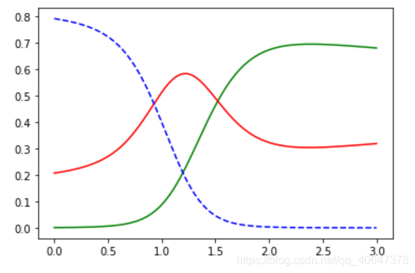
[2 1]

可以看出随着宽度的增加，结果在发生变化最后变成绿色
这个是单维的根据宽度

#逻辑回归的多分类转换成多个二分类详解
改用所有的特征
multi_class:
ovr :把多分类问题转换为多个二分类问题
multinomimal：是把多分类问题转换为 softmax问题，之后再讲

import numpy as np
from sklearn import datasets
from sklearn.linear_model import LogisticRegression
from sklearn.model_selection import GridSearchCV
#import matplotlib as plt
import matplotlib.pyplot as plt
from time import time

iris=datasets.load_iris()
x=iris['data'] 

print(iris['target'])
y=iris['target']
print(y)

start=time()
param_grid={"tol":[1e-4,1e-3,1e-2],
           "c":[0.4,0.6,0.8]}
log_reg=LogisticRegression(multi_class='ovr',solver='sag')
#log_reg=LogisticRegression(multi_class='ovr',solver='sag',max_iter=10000)
log_reg.fit(x, y)
grid_search=GridSearchCV(log_reg,param_grid=param_grid,cv=3)

print("w1",log_reg.coef_)
print("w0",log_reg.intercept_)

#结果  可以看到是四个维度
[0 0 0 0 0 0 0 0 0 0 0 0 0 0 0 0 0 0 0 0 0 0 0 0 0 0 0 0 0 0 0 0 0 0 0 0 0
 0 0 0 0 0 0 0 0 0 0 0 0 0 1 1 1 1 1 1 1 1 1 1 1 1 1 1 1 1 1 1 1 1 1 1 1 1
 1 1 1 1 1 1 1 1 1 1 1 1 1 1 1 1 1 1 1 1 1 1 1 1 1 1 2 2 2 2 2 2 2 2 2 2 2
 2 2 2 2 2 2 2 2 2 2 2 2 2 2 2 2 2 2 2 2 2 2 2 2 2 2 2 2 2 2 2 2 2 2 2 2 2
 2 2]
[0 0 0 0 0 0 0 0 0 0 0 0 0 0 0 0 0 0 0 0 0 0 0 0 0 0 0 0 0 0 0 0 0 0 0 0 0
 0 0 0 0 0 0 0 0 0 0 0 0 0 1 1 1 1 1 1 1 1 1 1 1 1 1 1 1 1 1 1 1 1 1 1 1 1
 1 1 1 1 1 1 1 1 1 1 1 1 1 1 1 1 1 1 1 1 1 1 1 1 1 1 2 2 2 2 2 2 2 2 2 2 2
 2 2 2 2 2 2 2 2 2 2 2 2 2 2 2 2 2 2 2 2 2 2 2 2 2 2 2 2 2 2 2 2 2 2 2 2 2
 2 2]
w1 [[ 0.31106995  1.39865099 -2.26183318 -1.015599  ]
 [ 0.167201   -1.82187685  0.62483746 -1.34699512]
 [-1.39111251 -1.30914738  2.50896799  2.50261786]]
w0 [ 0.9995961   2.99826938 -3.96230674]
C:\ProgramData\Anaconda3\lib\site-packages\sklearn\linear_model\sag.py:337: ConvergenceWarning: The max_iter was reached which means the coef_ did not converge
  "the coef_ did not converge", ConvergenceWarning)

#这个是警告没有收敛，可以改上面的迭代的次数

或许快要下雪了吧

发布了39 篇原创文章 · 获赞 1 · 访问量 472

私信关注

【放假第2天】人工智能-逻辑回归多分类-代码

Iris plants dataset

猜你喜欢