时间序列预测

参考：

• https://tensorflow.google.cn/tutorials/structured_data/time_series

一、时间序列预测

1.1、数据集

#显示所有列(参数设置为None代表显示所有行，也可以自行设置数字)
pd.set_option('display.max_columns',None)
#禁止自动换行(设置为Flase不自动换行，True反之)
pd.set_option('expand_frame_repr', False)

def loadWeatherData():
    # 如果直接下载不了，将提前下载好的数据集放到指定的dataset目录(xx\.keras\datasets\)
    zip_path = tf.keras.utils.get_file(
        origin='https://storage.googleapis.com/tensorflow/tf-keras-datasets/jena_climate_2009_2016.csv.zip',
        fname='jena_climate_2009_2016.csv.zip',
        extract=True)
    csv_path, _ = os.path.splitext(zip_path)
    print(csv_path)

    # 使用pands读取csv文件
    df = pd.read_csv(csv_path)
    print(df.head())

每10分钟一条记录

如上所示，每10分钟记录一次观察。这意味着，在一个小时内，你将有6次观察。同样，一天将包含144 (6x24)次观测。

给定一个特定的时间，假设你想预测未来6小时的温度。为了做出预测，你选择使用5天的观测。因此，您将创建一个包含最后720(5x144)次观察的窗口来训练模型。可能有许多这样的配置，这使这个数据集成为一个很好的实验对象。

下面的函数返回上面描述的模型训练时间窗口。参数history_size是信息的过去窗口的大小。target_size是需要预测的标签。

def univariate_data(dataset, start_index, end_index, history_size, target_size):
    '''
    dataset:
    start_index:
    end_index:
    history_size:
    target_size:

    @return: 特征, 标签
    '''

    data = []
    labels = []

    start_index = start_index + history_size
    if end_index is None:
        end_index = len(dataset) - target_size

    for i in range(start_index, end_index):
        indices = range(i-history_size, i)
        # Reshape data from (history_size,) to (history_size, 1)
        data.append(np.reshape(dataset[indices], (history_size, 1)))
        labels.append(dataset[i+target_size])

    return np.array(data), np.array(labels)

1.2、单一变量预测

1.2.1、提取单一便利，此例中提取温度

# 抽取单一变量， 此处为温度，以供使用预测
uni_data = df['T (degC)']
# 线性的数据结构, series是一个一维数组
# Pandas 会默然用0到n-1来作为series的index, 但也可以自己指定index( 可以把index理解为dict里面的key )
uni_data.index = df['Date Time']
print(type(uni_data), '\n' ,uni_data.head())

数据可视化

#可视化
uni_data.plot(subplots=True)
plt.show()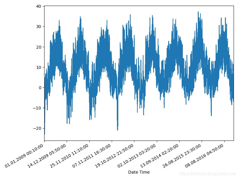

1.2.2、数据集归一化

Note: The mean and standard deviation should only be computed using the training data.

# 训练数据的平均及标准差
uni_train_mean = uni_data[:TRAIN_SPLIT].mean()
uni_train_std = uni_data[:TRAIN_SPLIT].std()

# 归一化
uni_data = (uni_data - uni_train_mean)/uni_train_std

1.2.3、拆分训练集与验证数据集

# 训练集
x_train_uni, y_train_uni = univariate_data(uni_data, 0, TRAIN_SPLIT,
                                           univariate_past_history,
                                           univariate_future_target)
# 验证集
x_val_uni, y_val_uni = univariate_data(uni_data, TRAIN_SPLIT, None,
                                   univariate_past_history,
                                   univariate_future_target)

print ('Single window of past history')
print (x_train_uni[0])
print ('\n Target temperature to predict')
print (y_train_uni[0])

下图中蓝色线是给网络训练的数据， 红色叉叉是要预测的数据

def create_time_steps(length):
    return list(range(-length, 0))

def baseline(history):
    return np.mean(history)

def show_plot(plot_data, delta, title):
    labels = ['History', 'True Future', 'Model Prediction']
    marker = ['.-', 'rx', 'go']
    time_steps = create_time_steps(plot_data[0].shape[0])
    if delta:
        future = delta
    else:
        future = 0

    plt.title(title)
    for i, x in enumerate(plot_data):
        if i:
            plt.plot(future, plot_data[i], marker[i], markersize=10,
                     label=labels[i])
        else:
            plt.plot(time_steps, plot_data[i].flatten(), marker[i], label=labels[i])
    plt.legend()
    plt.xlim([time_steps[0], (future+5)*2])
    plt.xlabel('Time-Step')
    return plt

show_plot([x_train_uni[0], y_train_uni[0]], 0, 'Sample Example')
plt.show()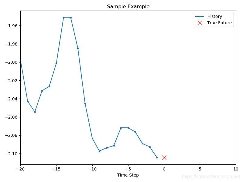

在继续训练模型之前，让我们首先设置一个简单的基线。给定一个输入点，基线方法查看所有历史记录，并预测下一个点是最近20个观察值的平均值。

show_plot([x_train_uni[0], y_train_uni[0], baseline(x_train_uni[0])], 0,
          'Baseline Prediction Example')
plt.show()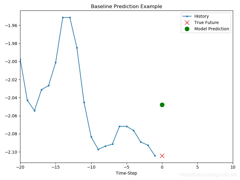

让我们看看你是否可以使用递归神经网络来超越这个基线。

1.2.4、 RNN

1.3、多变量预测