摘要:本文先从梯度下降法的理论推导开始,说明梯度下降法为什么能够求得函数的局部极小值。通过两个小例子,说明梯度下降法求解极限值实现过程。在通过分解BP神经网络,详细说明梯度下降法在神经网络的运算过程,并详细写出每一步的计算结果。该过程通俗易懂,有基本的高数和线代基础即可理解明白。最后通过tensorflow实现一个简单的线性回归,对照理解梯度下降法在神经网络中的应用。码字不易,转载请标明出处。该文中部分内容是研究生课堂论文内容,为避免课程论文被误解为抄袭,所用截图特意添加水印。
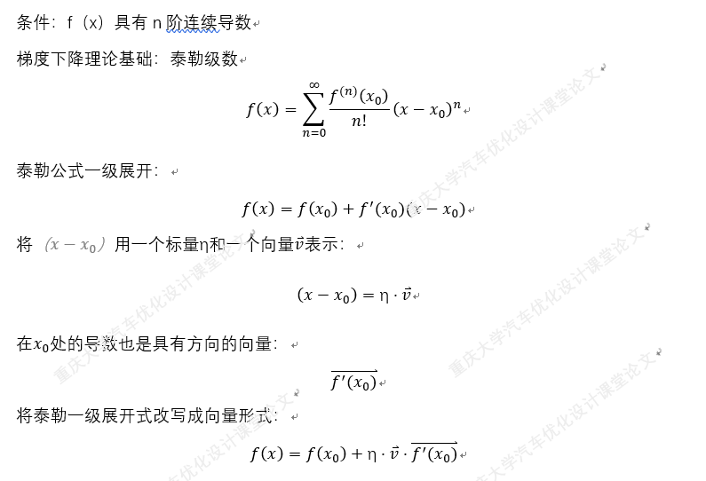
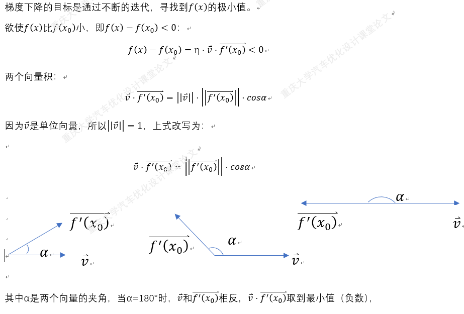
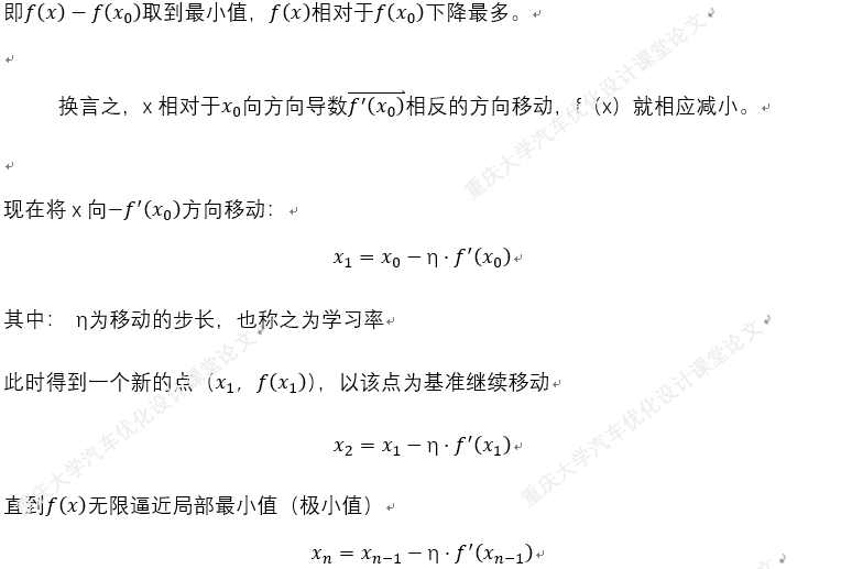
一.梯度下降法的理论推导:
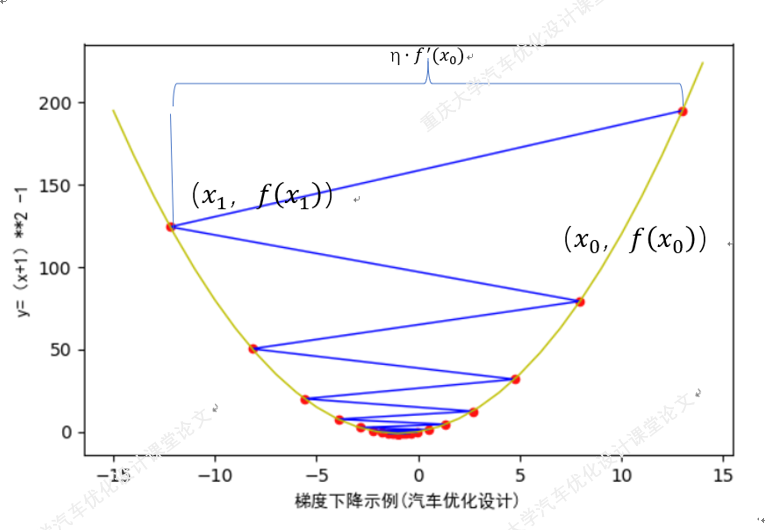
二.求解一个简单的一元函数极小值
例:求函数y=(x+1)^2-1的极小值:
实现环境:python3.6
相关模块:numpy 、 matplotlib


import numpy as np
from matplotlib import pyplot as plt
def function_1d(x):
    '''
    目标函数:求目标函数的极小值
    x:自变量,标量
    返回:因变量,标量
    '''
    return (x+1)**2-1
##2.定义梯度函数
def grad_1d(x):
    '''
    :param x: 自变量,标量
    :return: 因变量,标量
    '''
    return 2*(x+1)
##3.定义迭代过程
def gradient_descent_1d(grad,current_x,learning_rate=0.0001,precision=0.0001,max_iters=10000):
    '''
    一维问题的梯度下降法
    :param grad: 目标函数的梯度
    :param current_x: 当前x值
    :param learning_rate: 学习率=η
    :param precision: 收敛精度
    :param max_iters: 最大迭代次数
    :return: 极小值
    '''
    ##创建一个空列表用于接收每次移动后的current_x
    cur_x_list = []
    cur_x_list.append(current_x)
    for i in range(max_iters):
        grad_current = grad(current_x)
        if abs(grad_current)<precision:
            break            ##梯度小于收敛精度时,视为收敛
        current_x = current_x-grad_current*learning_rate
        cur_x_list.append(current_x)
        print('第%s次迭代:x=%s'%(i,current_x))
    print('极小值点(%s,%s)'%(current_x,function_1d(current_x)))
    return cur_x_list
##4.运行返回极小值和x移动轨迹
if __name__ == '__main__':
    cur_x_list = gradient_descent_1d(grad_1d,learning_rate=0.9,current_x=13)  ##开始梯度下降,并且返回每次变化后的x,学习率=η=0.9

    cur_x_array = np.array(cur_x_list)
    cur_y_array = function_1d(cur_x_array)
    ##绘制曲线图
    plt.figure(figsize=(6,4))
    plt.subplot()
    x = cur_x_array
    y = function_1d(x)
    plt.plot(x, y, color='b', linewidth=1)
    ##绘制函数图
    x1 = np.arange(-15,15,1)
    y1 = np.array(function_1d(x1))
    plt.plot(x1, y1, color='y', linewidth=1)
    ##散点图
    plt.scatter(cur_x_array,cur_y_array,s=20,c="#ff1212",marker='o')
    plt.xlabel('梯度下降示例(汽车优化设计)',fontproperties = 'SimHei',fontsize = 10)
    plt.ylabel('y=(x+1)**2 -1',fontproperties = 'SimHei',fontsize = 10)
    plt.show()


###输出结果
第0次迭代:x=-12.2
第1次迭代:x=7.960000000000001
第2次迭代:x=-8.168000000000003
第3次迭代:x=4.734400000000003
第4次迭代:x=-5.587520000000003
第5次迭代:x=2.670016000000002
第6次迭代:x=-3.936012800000002
第7次迭代:x=1.3488102400000015
第8次迭代:x=-2.8790481920000017
第9次迭代:x=0.5032385536000015
第10次迭代:x=-2.202590842880001
第11次迭代:x=-0.03792732569599888
第12次迭代:x=-1.769658139443201
第13次迭代:x=-0.3842734884454393
第14次迭代:x=-1.4925812092436486
第15次迭代:x=-0.6059350326050811
第16次迭代:x=-1.3152519739159352
第17次迭代:x=-0.7477984208672518
第18次迭代:x=-1.2017612633061985
第19次迭代:x=-0.8385909893550412
第20次迭代:x=-1.1291272085159672
第21次迭代:x=-0.8966982331872263
第22次迭代:x=-1.082641413450219
第23次迭代:x=-0.9338868692398249
第24次迭代:x=-1.05289050460814
第25次迭代:x=-0.957687596313488
第26次迭代:x=-1.0338499229492095
第27次迭代:x=-0.9729200616406324
第28次迭代:x=-1.021663950687494
第29次迭代:x=-0.9826688394500047
第30次迭代:x=-1.0138649284399963
第31次迭代:x=-0.9889080572480029
第32次迭代:x=-1.0088735542015976
第33次迭代:x=-0.9929011566387219
第34次迭代:x=-1.0056790746890225
第35次迭代:x=-0.995456740248782
第36次迭代:x=-1.0036346078009744
第37次迭代:x=-0.9970923137592205
第38次迭代:x=-1.0023261489926236
第39次迭代:x=-0.9981390808059011
第40次迭代:x=-1.001488735355279
第41次迭代:x=-0.9988090117157767
第42次迭代:x=-1.0009527906273785
第43次迭代:x=-0.9992377674980972
第44次迭代:x=-1.0006097860015222
第45次迭代:x=-0.9995121711987822
第46次迭代:x=-1.0003902630409742
第47次迭代:x=-0.9996877895672206
第48次迭代:x=-1.0002497683462235
第49次迭代:x=-0.9998001853230212
第50次迭代:x=-1.000159851741583
第51次迭代:x=-0.9998721186067335
第52次迭代:x=-1.0001023051146132
第53次迭代:x=-0.9999181559083095
第54次迭代:x=-1.0000654752733524
第55次迭代:x=-0.9999476197813181
第56次迭代:x=-1.0000419041749455
极小值点(-1.0000419041749455,-0.9999999982440401)

Process finished with exit code 0
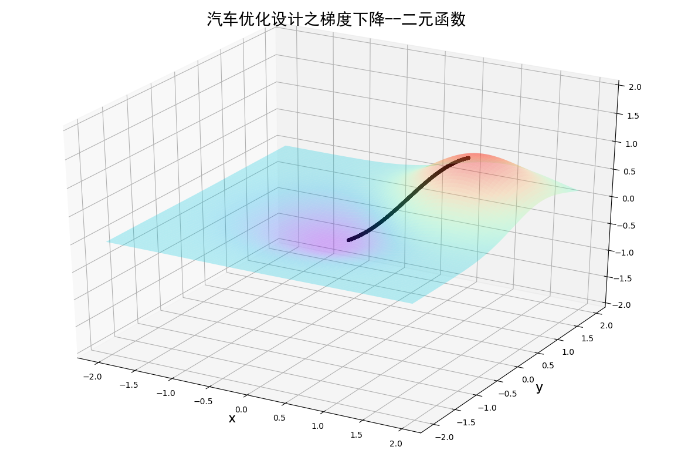
三.求解一个简单的二元函数的极小值

import numpy as np
from tqdm import tqdm
from matplotlib import pyplot as plt
from mpl_toolkits.mplot3d import  Axes3D
def plot_3d():
    fig = plt.figure(figsize=(12,8))
    ax = Axes3D(fig)
    x = np.arange(-3,3,0.1)
    y = np.arange(-3,3,0.1)
    ##对x,y数据执行网格化
    x,y = np.meshgrid(x,y)
    z = -(z1-2*z2)*0.1
    ax.plot_surface(x,y,z,
                    rstride=1,##retride(row)指定行的跨度
                    cstride=1,##retride(column)指定列的跨度
                    cmap='rainbow')  ##设置颜色映射
    ##设置z轴范围
    ax.set_zlim(-2,2)
    ##设置标题
    plt.title('汽车优化设计之梯度下降--目标函数',fontproperties = 'SimHei',fontsize = 20)
    plt.show()
# plot_3d()


'''二维梯度下降法'''
def func_2d_single(x,y):
    '''
    目标函数传入x,y
    :param x,y: 自变量,一维向量
    :return: 因变量,标量
    '''
    z1 = np.exp(-x**2-y**2)
    z2 = np.exp(-(x-1)**2-(y-1)**2)
    z = -(z1-2*z2)*0.5
    return z
def plot_3d():
    fig = plt.figure(figsize=(12,8))
    ax = Axes3D(fig)
    x = np.arange(-3,3,0.1)
    y = np.arange(-3,3,0.1)
    ##对x,y数据执行网格化
    x,y = np.meshgrid(x,y)
    z = func_2d_single(x,y)
    ax.plot_surface(x,y,z,
                    rstride=1,##retride(row)指定行的跨度
                    cstride=1,##retride(column)指定列的跨度
                    cmap='rainbow')  ##设置颜色映射
    ##设置z轴范围
    ax.set_zlim(-2,2)
    ##设置标题
    plt.title('汽车优化设计之梯度下降--目标函数3维图',fontproperties = 'SimHei',fontsize = 20)
    plt.show()
plot_3d()

def func_2d(xy):
    '''
    目标函数传入xy组成的数组,如[x1,y1]
    :param xy: 自变量,二维向量  (x,y)
    :return: 因变量,标量
    '''
    z1 = np.exp(-xy[0]**2-xy[1]**2)
    z2 = np.exp(-(xy[0]-1)**2-(xy[1]-1)**2)
    z = -(z1-2*z2)*0.5
    return z
def grad_2d(xy):
    '''
    目标函数的梯度
    :param xy: 自变量,二维向量
    :return: 因变量,二维向量  (分别求偏导数,组成数组返回)
    '''
    grad_x = 2*xy[0]*(np.exp(-(xy[0]**2+xy[1]**2)))
    grad_y = 2*xy[1]*(np.exp(-(xy[0]**2+xy[1]**2)))
    return np.array([grad_x,grad_y])
def gradient_descent_2d(grad, cur_xy=np.array([1, 1]), learning_rate=0.001, precision=0.001, max_iters=100000000):
    '''
    二维目标函数的梯度下降法
    :param grad: 目标函数的梯度
    :param cur_xy: 当前的x和y值
    :param learning_rate: 学习率
    :param precision: 收敛精度
    :param max_iters: 最大迭代次数
    :return: 返回极小值
    '''
    print(f"{cur_xy} 作为初始值开始的迭代......")
    x_cur_list = []
    y_cur_list = []
    for i in tqdm(range(max_iters)):
        grad_cur = grad(cur_xy)
        ##创建两个列表,用于接收变化的x,y
        x_cur_list.append(cur_xy[0])
        y_cur_list.append(cur_xy[1])
        if np.linalg.norm(grad_cur,ord=2)<precision:  ##求范数,ord=2 平方和开根
            break    ###当梯度接近于0时,视为收敛
        cur_xy = cur_xy-grad_cur*learning_rate
        x_cur_list.append(cur_xy[0])
        y_cur_list.append(cur_xy[1])
        print('第%s次迭代:x,y = %s'%(i,cur_xy))
    print('极小值 x,y = %s '%cur_xy)
    return (x_cur_list,y_cur_list)
if __name__=="__main__":
    current_xy_list = gradient_descent_2d(grad_2d)
    fig = plt.figure(figsize=(12,8))
    ax = Axes3D(fig)
    a = np.array(current_xy_list[0])
    b = np.array(current_xy_list[1])
    c = func_2d_single(a,b)
    ax.scatter(a,b,c,c='Black',s=10,alpha=1,marker='o')
    x = np.arange(-2,2,0.05)
    y = np.arange(-2,2,0.05)
    ##对x,y数据执行网格化
    x,y = np.meshgrid(x,y)
    z = func_2d_single(x,y)
    ax.plot_surface(x,y,z,
                    rstride=1,##retride(row)指定行的跨度
                    cstride=1,##retride(column)指定列的跨度
                    cmap='rainbow',
                    alpha=0.3
                    )  ##设置颜色映射
    # ax.plot_wireframe(x,y,z,)
    ##设置z轴范围
    ax.set_zlim(-2,2)
    ##设置标题
    plt.title('汽车优化设计之梯度下降--二元函数',fontproperties = 'SimHei',fontsize = 20)
    plt.xlabel('x',fontproperties = 'SimHei',fontsize = 20)
    plt.ylabel('y', fontproperties='SimHei', fontsize=20)
    plt.show()
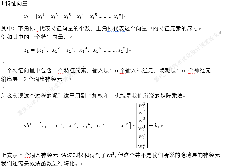
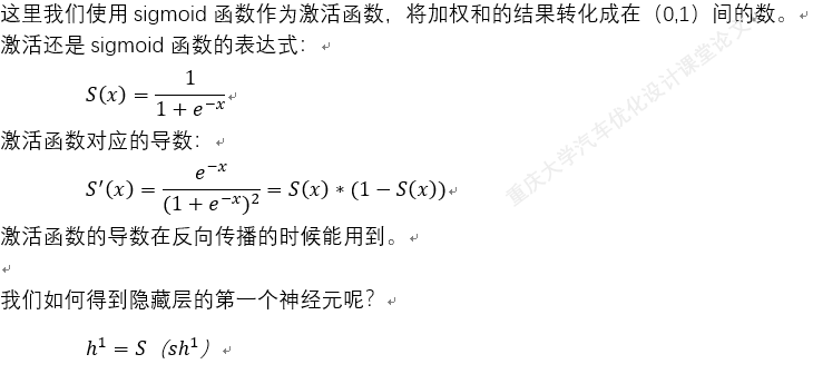
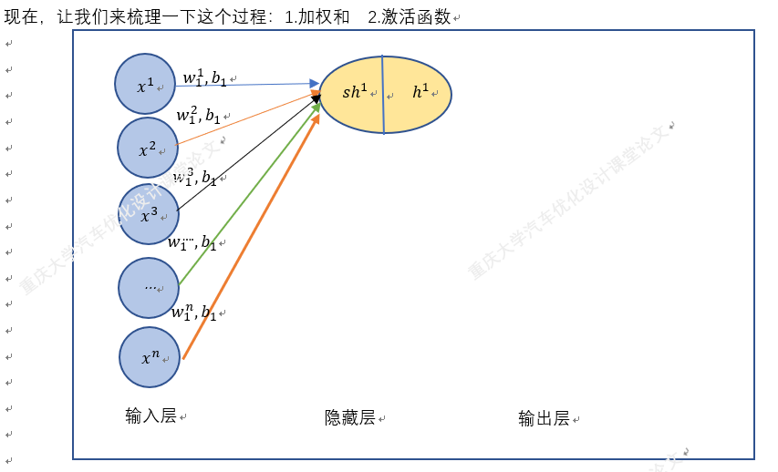
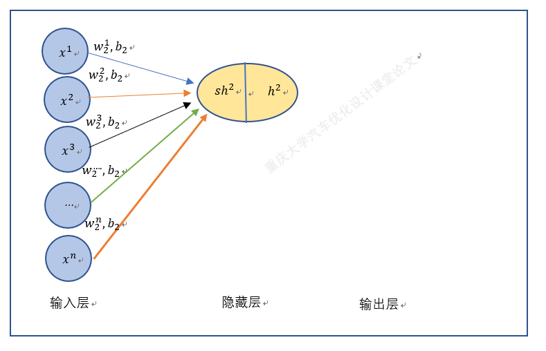
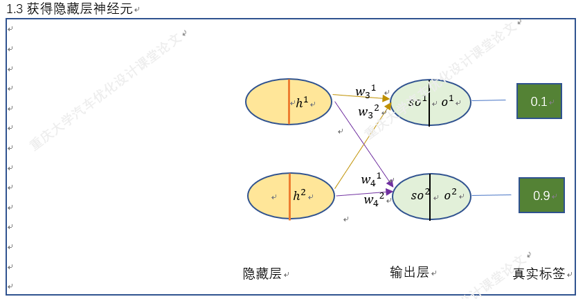
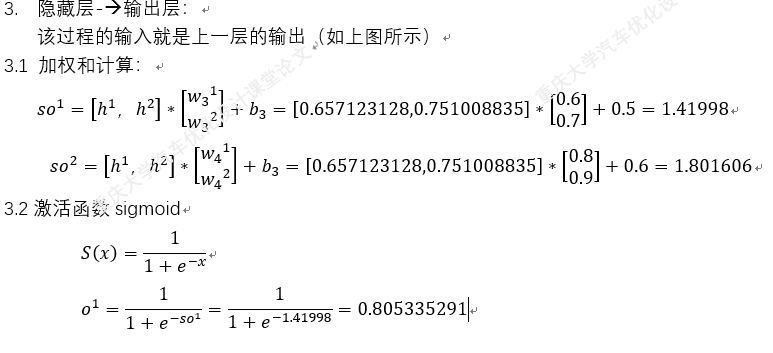
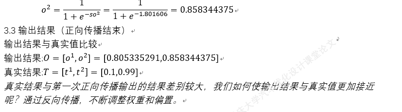
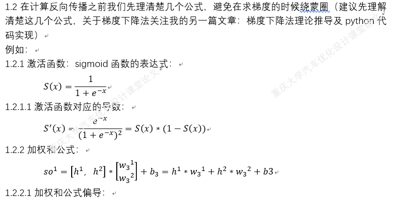
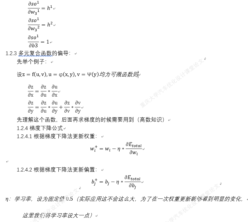
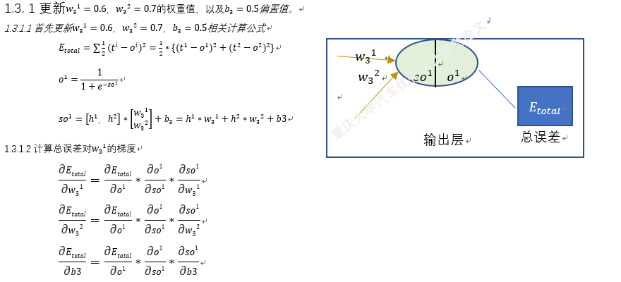
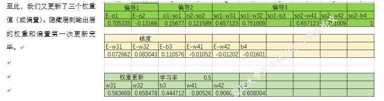
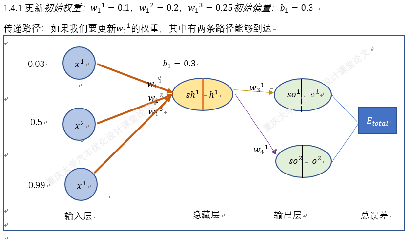
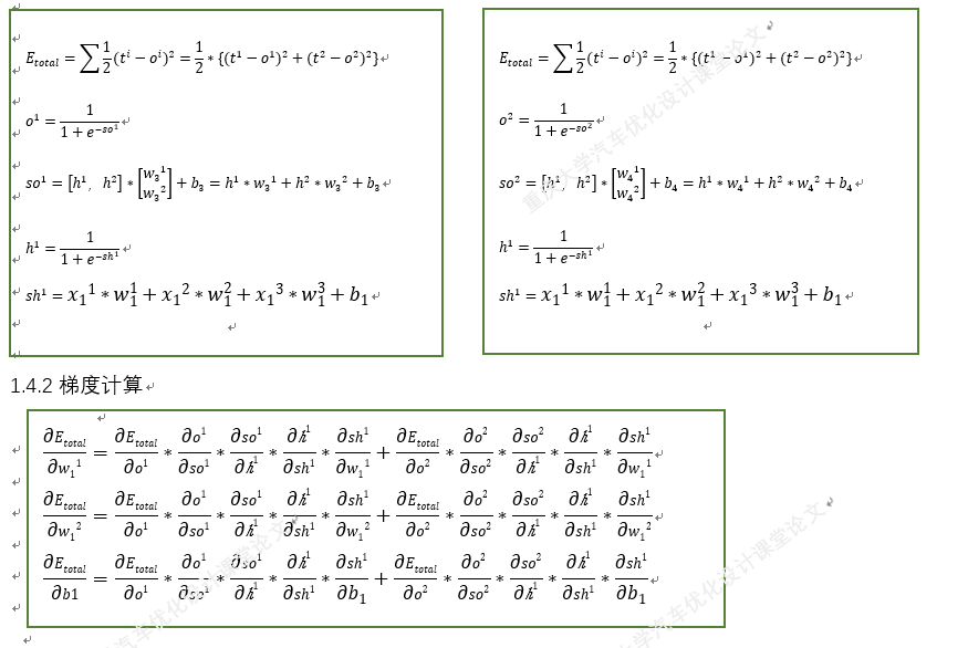
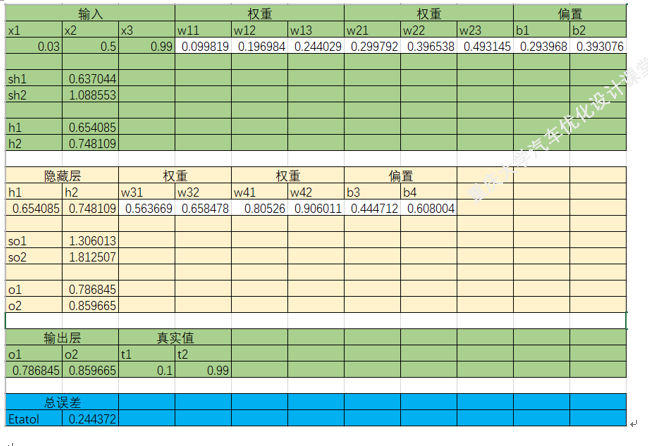
四.梯度下降法在BP神经网络中的实现过程(手动+Excel处理)
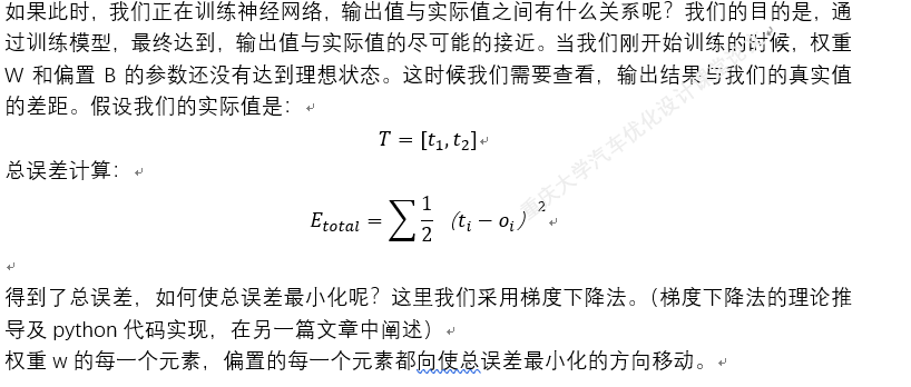
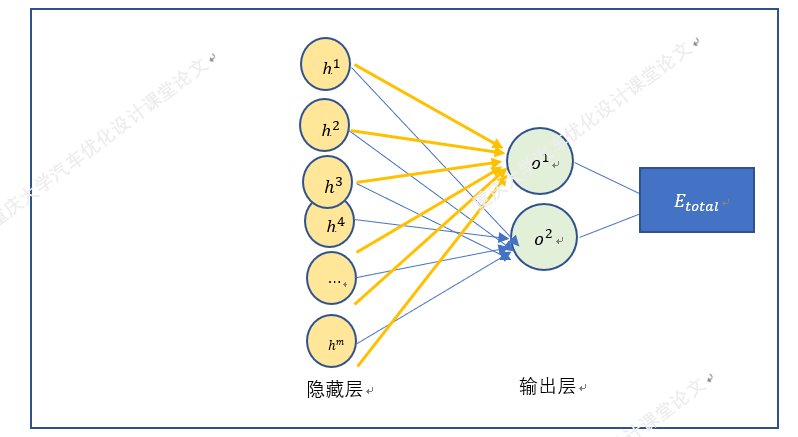
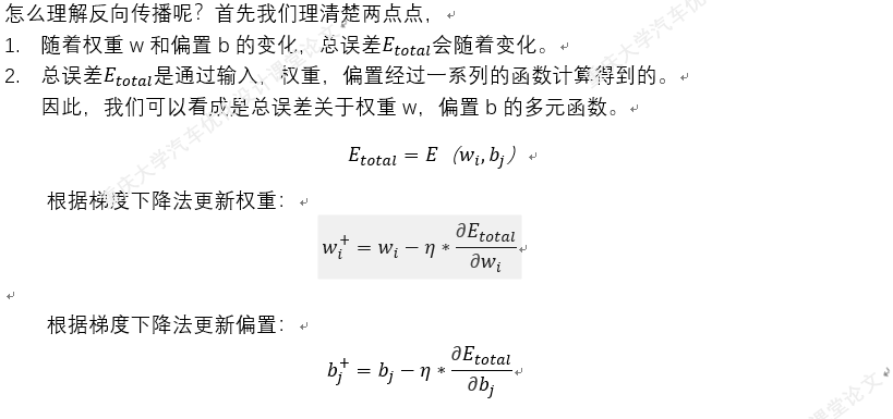
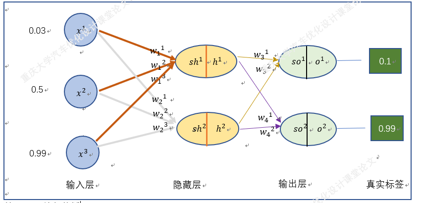
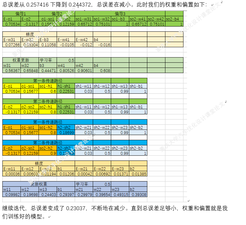
BP神经网络中的正向传播和反向传播过程。反向传播中的权重更新,就是通过梯度下降法实现的,损失函数最小化,实质也是一个最优化问题的求解。


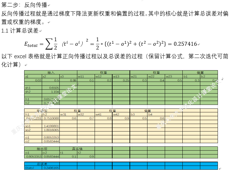

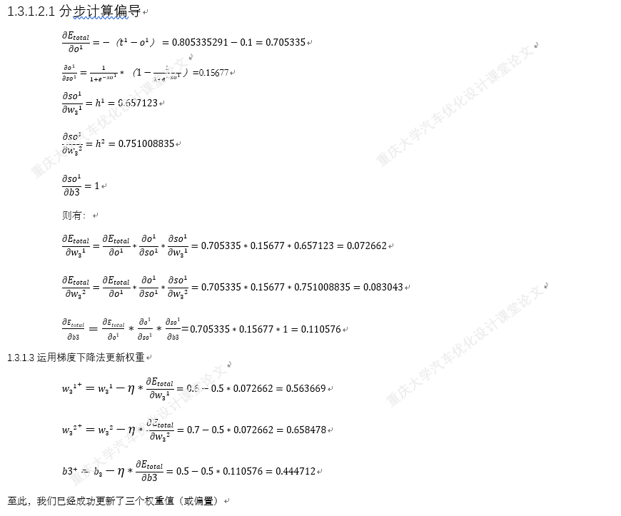


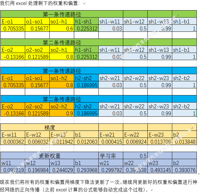

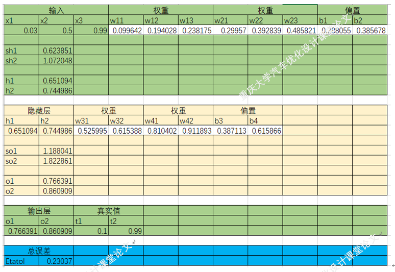
以上就是BP神经网络的实现过程,手动+excel码字只是为了深刻理解神经网络,但这个并没有太大的实质性意义,因为这个已经是成熟的算法。
五.Tensorflow中实现简单的线性回归