In numerical methods, we can reduce dt or dx to improve the accuracy of solving equations and calculating integration. However, it will also increase the time cost. Here we show some examples to obtain results with Higher accuracy and Less time cost.
(1) Lagrange Method
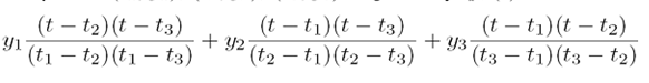
Similar to the linear interpolation, we can construct a quadratic polynomial with three points (t1, y1), (t2, y2), (t3, y3). In Octave, we can use the spline function for interpolation.


Suppose we have the raw data(x,y) with 11 points (plot with blue circle). xx=linspace(0,10); yy=spline(x,y,xx); We will obtain the curve(plot in red line) which is interpolated from (x,y) using the spline function.
(2) Simpson Quadrature
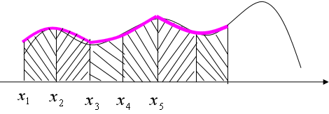
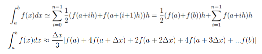
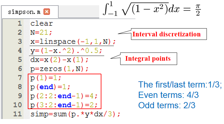
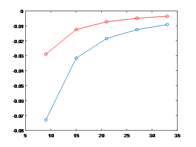
In Trapezoidal Quadrature, the first and last terms are1/2, and other terms are 1. We can tune the weight parameters to improve accuracy. In Simpson method, the first/last terms are1/3, while other even terms are 4/3 and other odd terms are 2/3. As shown below, the red line is the result of Simpson, whose accuracy is better than that of Trapezoidal Quadrature(blue line).
(3) Fitting-Least Square Method
For interpolation, we do not know the form of function while we can choose a proper function with parameters to fit data. The parameters can be further determined by Least Square Method. For a linear fitting, the slope (A_1) and constant (A_0) can be calculated from the data.

In Octave, we can use the function of polyfit. With the total energies of Diamond nanocrystals, we can find the linear dependence of E_tot per carbon on the H/C ratio.
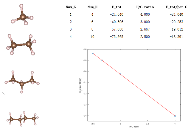
clear
a=[4.000 	-24.040
3.000 	-20.253
2.667 	-19.012
2.500 	-18.391
];
plot(a(:,1),a(:,2),'o')
q=polyfit(a(:,1),a(:,2),1);
x=linspace(min(a(:,1)),max(a(:,1)));
hold on
plot(x,q(1)*x+q(2),'r')
xlabel('H/C ratio')
ylabel('E_tot per C(eV)')