C4W1：Convolutional Neural Networks: Application

原文链接： https://www.jianshu.com/p/f19e68266008

目标

• 完成一些辅助函数
• 使用 TensorFlow 实现一个 ConvNet，用于解决分类问题

1. 准备工作

1.1 导入相关包

import math
import numpy as np
import h5py
import matplotlib.pyplot as plt
import scipy
from PIL import Image
from scipy import ndimage
import tensorflow as tf
from tensorflow.python.framework import ops
from cnn_utils import *

%matplotlib inline
np.random.seed(1)

1.2 加载数据集

使用如下命令加载 SIGNS 数据集：SIGNS 数据集包含了从 0 到 5 的六个数字。

# Loading the data (signs)
X_train_orig, Y_train_orig, X_test_orig, Y_test_orig, classes = load_dataset()

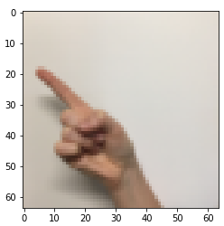
下面展示了数据集的样本及其对应的标签，改变 index 的值可以看到不同的数据：

# Example of a picture
index = 7
plt.imshow(X_train_orig[index])
print ("y = " + str(np.squeeze(Y_train_orig[:, index])))

>>>
y = 1

1.3 查看数据格式

X_train = X_train_orig/255.
X_test = X_test_orig/255.
Y_train = convert_to_one_hot(Y_train_orig, 6).T
Y_test = convert_to_one_hot(Y_test_orig, 6).T
print ("number of training examples = " + str(X_train.shape[0]))
print ("number of test examples = " + str(X_test.shape[0]))
print ("X_train shape: " + str(X_train.shape))
print ("Y_train shape: " + str(Y_train.shape))
print ("X_test shape: " + str(X_test.shape))
print ("Y_test shape: " + str(Y_test.shape))
conv_layers = {}

>>>
number of training examples = 1080
number of test examples = 120
X_train shape: (1080, 64, 64, 3)
Y_train shape: (1080, 6)
X_test shape: (120, 64, 64, 3)
Y_test shape: (120, 6)

2. TensorFlow 模型

2.1 创建 placeholders

TensorFlow 要求我们为输入数据创建 placeholders，以便在运行 session 时将输入数据喂入模型中。

要求：为输入数据 X 和输出数据 Y 创建 placeholders，对于 batch size 可以先设置为 None。所以输入 X 的形状为 (None, n_H0, n_W0, n_C0)，Y的形状为 (None, n_y)。

# GRADED FUNCTION: create_placeholders

def create_placeholders(n_H0, n_W0, n_C0, n_y):
    """
    Creates the placeholders for the tensorflow session.

    Arguments:
    n_H0 -- scalar, height of an input image
    n_W0 -- scalar, width of an input image
    n_C0 -- scalar, number of channels of the input
    n_y -- scalar, number of classes

    Returns:
    X -- placeholder for the data input, of shape [None, n_H0, n_W0, n_C0] and dtype "float"
    Y -- placeholder for the input labels, of shape [None, n_y] and dtype "float"
    """

    ### START CODE HERE ### (≈2 lines)
    X = tf.placeholder(tf.float32,shape=(None,n_H0,n_W0,n_C0))
    Y = tf.placeholder(tf.float32,shape=(None,n_y))
    ### END CODE HERE ###

    return X, Y

X, Y = create_placeholders(64, 64, 3, 6)
print ("X = " + str(X))
print ("Y = " + str(Y))

>>>
X = Tensor("Placeholder:0", shape=(?, 64, 64, 3), dtype=float32)
Y = Tensor("Placeholder_1:0", shape=(?, 6), dtype=float32)

2.2 初始化参数

使用 tf.contrib.layers.xavier_initializer(seed = 0) 初始化权重（卷积核） $W1$ 和 $W2$，这里不需要考虑偏置 bias，因为 TensorFlow 的函数已经对 bias 做了处理，所以只需要初始化权重。同时 TensorFlow 自动对全连接层做初始化。

提示：如果想要初始化一个形状为 [1, 2, 3, 4] 的参数 $W$，在 TensorFlow 中可以这样做：

W = tf.get_variable("W", [1,2,3,4], initializer = ...)

# GRADED FUNCTION: initialize_parameters

def initialize_parameters():
    """
    Initializes weight parameters to build a neural network with tensorflow. The shapes are:
                        W1 : [4, 4, 3, 8]
                        W2 : [2, 2, 8, 16]
    Returns:
    parameters -- a dictionary of tensors containing W1, W2
    """
    
    tf.set_random_seed(1)                              # so that your "random" numbers match ours
        
    ### START CODE HERE ### (approx. 2 lines of code)
    W1 = tf.get_variable('W1',[4,4,3,8],initializer=tf.contrib.layers.xavier_initializer(seed = 0))
    W2 = tf.get_variable('W2',[2,2,8,16],initializer=tf.contrib.layers.xavier_initializer(seed = 0))
    ### END CODE HERE ###

    parameters = {"W1": W1,
                  "W2": W2}
    
    return parameters

tf.reset_default_graph()
with tf.Session() as sess_test:
    parameters = initialize_parameters()
    init = tf.global_variables_initializer()
    sess_test.run(init)
    print("W1 = " + str(parameters["W1"].eval()[1,1,1]))
    print("W2 = " + str(parameters["W2"].eval()[1,1,1]))

>>>
W1 = [ 0.00131723  0.1417614  -0.04434952  0.09197326  0.14984085 -0.03514394
 -0.06847463  0.05245192]
W2 = [-0.08566415  0.17750949  0.11974221  0.16773748 -0.0830943  -0.08058
 -0.00577033 -0.14643836  0.24162132 -0.05857408 -0.19055021  0.1345228
 -0.22779644 -0.1601823  -0.16117483 -0.10286498]

2.3 前向传播

在 TensorFlow 中，有许多内置的函数实现卷积操作：

• tf.nn.conv2d(X,W1, strides = [1,s,s,1], padding = 'SAME')：给出输入 $X$ 和一组卷积核 $W1$，该函数可以实现将 $W1$ 在 $X$ 上进行卷积。第 3 个输入参数表示步长 [详细说明]
• tf.nn.max_pool(A, ksize = [1,f,f,1], strides = [1,s,s,1], padding = 'SAME')：给出输入 $A$，该函数会使用大小为 (f,f) 的窗口和 (s,s) 的步长来做最大池化 [详细说明]
• tf.nn.relu(Z1)：计算 $Z1$ 的 Relu 输出 [详细说明]
• tf.contrib.layers.flatten(P)：给出输入 $P$，该函数会将其变为一维向量，返回一个形状为 [batch_size, k] 的 tensor [详细说明]
• tf.contrib.layers.fully_connected(F, num_outputs)：给出一个输入 F，该函数计算经过全连接层之后的输出结果，且自动初始化权重参数 [详细说明]

建立前向传播：CONV2D -> RELU -> MAXPOOL -> CONV2D -> RELU -> MAXPOOL -> FLATTEN -> FULLYCONNECTED

提示：在每一步会用到以下参数

• Conv2D: stride 1, padding is “SAME”
• ReLU
• Max pool: Use an 8 by 8 filter size and an 8 by 8 stride, padding is “SAME”
• Conv2D: stride 1, padding is “SAME”
• ReLU
• Max pool: Use a 4 by 4 filter size and a 4 by 4 stride, padding is “SAME”
• Flatten the previous output

# GRADED FUNCTION: forward_propagation

def forward_propagation(X, parameters):
    """
    Implements the forward propagation for the model:
    CONV2D -> RELU -> MAXPOOL -> CONV2D -> RELU -> MAXPOOL -> FLATTEN -> FULLYCONNECTED
    
    Arguments:
    X -- input dataset placeholder, of shape (input size, number of examples)
    parameters -- python dictionary containing your parameters "W1", "W2"
                  the shapes are given in initialize_parameters

    Returns:
    Z3 -- the output of the last LINEAR unit
    """
    
    # Retrieve the parameters from the dictionary "parameters" 
    W1 = parameters['W1']
    W2 = parameters['W2']
    
    ### START CODE HERE ###
    # CONV2D: stride of 1, padding 'SAME'
    Z1 = tf.nn.conv2d(X,W1, strides = [1,1,1,1], padding = 'SAME')
    # RELU
    A1 = tf.nn.relu(Z1)
    # MAXPOOL: window 8x8, sride 8, padding 'SAME'
    P1 = tf.nn.max_pool(A1, ksize = [1,8,8,1], strides = [1,8,8,1], padding = 'SAME')
    # CONV2D: filters W2, stride 1, padding 'SAME'
    Z2 = tf.nn.conv2d(P1,W2, strides = [1,1,1,1], padding = 'SAME')
    # RELU
    A2 = tf.nn.relu(Z2)
    # MAXPOOL: window 4x4, stride 4, padding 'SAME'
    P2 = tf.nn.max_pool(A2, ksize = [1,4,4,1], strides = [1,4,4,1], padding = 'SAME')
    # FLATTEN
    P2 = tf.contrib.layers.flatten(P2)
    # FULLY-CONNECTED without non-linear activation function (not not call softmax).
    # 6 neurons in output layer. Hint: one of the arguments should be "activation_fn=None" 
    Z3 = tf.contrib.layers.fully_connected(P2, num_outputs = 6, activation_fn=None)
    ### END CODE HERE ###

    return Z3

tf.reset_default_graph()

with tf.Session() as sess:
    np.random.seed(1)
    X, Y = create_placeholders(64, 64, 3, 6)
    parameters = initialize_parameters()
    Z3 = forward_propagation(X, parameters)
    init = tf.global_variables_initializer()
    sess.run(init)
    a = sess.run(Z3, {X: np.random.randn(2,64,64,3), Y: np.random.randn(2,6)})
    print("Z3 = " + str(a))

>>>
Z3 = [[-0.44670227 -1.5720876  -1.5304923  -2.3101304  -1.2910438   0.46852064]
 [-0.17601591 -1.5797201  -1.4737016  -2.616721   -1.0081065   0.5747785 ]]

2.4 计算 cost

计算损失时，可以使用 TensorFlow 中的两个函数：

• tf.nn.softmax_cross_entropy_with_logits(logits = Z3, labels = Y：计算 sofrmax entropy loss [详细说明]
• tf.reduce_mean：计算一个 tensor 中所有元素的平均值 [详细说明]

# GRADED FUNCTION: compute_cost 

def compute_cost(Z3, Y):
    """
    Computes the cost
    
    Arguments:
    Z3 -- output of forward propagation (output of the last LINEAR unit), of shape (6, number of examples)
    Y -- "true" labels vector placeholder, same shape as Z3
    
    Returns:
    cost - Tensor of the cost function
    """
    
    ### START CODE HERE ### (1 line of code)
    cost = tf.reduce_mean(tf.nn.softmax_cross_entropy_with_logits(logits = Z3, labels = Y))
    ### END CODE HERE ###
    
    return cost

tf.reset_default_graph()

with tf.Session() as sess:
    np.random.seed(1)
    X, Y = create_placeholders(64, 64, 3, 6)
    parameters = initialize_parameters()
    Z3 = forward_propagation(X, parameters)
    cost = compute_cost(Z3, Y)
    init = tf.global_variables_initializer()
    sess.run(init)
    a = sess.run(cost, {X: np.random.randn(4,64,64,3), Y: np.random.randn(4,6)})
    print("cost = " + str(a))

>>>
cost = 2.9103396

2.5 建立模型

使用上面已经写好的辅助函数来建立最终的模型，并将模型在 SIGNS 数据集上进行训练。模型需要 1）创建 placeholders，2）初始化参数，3）前向传播，4）计算损失，5）创建 optimizer，最后创建一个 session 并执行 num_epochs 次 for loop，在每一个 mini-batch 中都要对函数进行优化。

提示：random_mini_batches() 函数会返回一个 mini-batches 的列表

# GRADED FUNCTION: model

def model(X_train, Y_train, X_test, Y_test, learning_rate = 0.009,
          num_epochs = 100, minibatch_size = 64, print_cost = True):
    """
    Implements a three-layer ConvNet in Tensorflow:
    CONV2D -> RELU -> MAXPOOL -> CONV2D -> RELU -> MAXPOOL -> FLATTEN -> FULLYCONNECTED
    
    Arguments:
    X_train -- training set, of shape (None, 64, 64, 3)
    Y_train -- test set, of shape (None, n_y = 6)
    X_test -- training set, of shape (None, 64, 64, 3)
    Y_test -- test set, of shape (None, n_y = 6)
    learning_rate -- learning rate of the optimization
    num_epochs -- number of epochs of the optimization loop
    minibatch_size -- size of a minibatch
    print_cost -- True to print the cost every 100 epochs
    
    Returns:
    train_accuracy -- real number, accuracy on the train set (X_train)
    test_accuracy -- real number, testing accuracy on the test set (X_test)
    parameters -- parameters learnt by the model. They can then be used to predict.
    """
    
    ops.reset_default_graph()                         # to be able to rerun the model without overwriting tf variables
    tf.set_random_seed(1)                             # to keep results consistent (tensorflow seed)
    seed = 3                                          # to keep results consistent (numpy seed)
    (m, n_H0, n_W0, n_C0) = X_train.shape             
    n_y = Y_train.shape[1]                            
    costs = []                                        # To keep track of the cost
    
    # Create Placeholders of the correct shape
    ### START CODE HERE ### (1 line)
    X, Y = create_placeholders(n_H0,n_W0,n_C0,n_y)
    ### END CODE HERE ###

    # Initialize parameters
    ### START CODE HERE ### (1 line)
    parameters = initialize_parameters()
    ### END CODE HERE ###
    
    # Forward propagation: Build the forward propagation in the tensorflow graph
    ### START CODE HERE ### (1 line)
    Z3 = forward_propagation(X,parameters)
    ### END CODE HERE ###
    
    # Cost function: Add cost function to tensorflow graph
    ### START CODE HERE ### (1 line)
    cost = compute_cost(Z3,Y)
    ### END CODE HERE ###
    
    # Backpropagation: Define the tensorflow optimizer. Use an AdamOptimizer that minimizes the cost.
    ### START CODE HERE ### (1 line)
    optimizer = tf.train.AdamOptimizer(learning_rate = learning_rate).minimize(cost)
    ### END CODE HERE ###
    
    # Initialize all the variables globally
    init = tf.global_variables_initializer()
     
    # Start the session to compute the tensorflow graph
    with tf.Session() as sess:
        
        # Run the initialization
        sess.run(init)
        
        # Do the training loop
        for epoch in range(int(num_epochs)):

            minibatch_cost = 0.
            num_minibatches = int(m / minibatch_size) # number of minibatches of size minibatch_size in the train set
            seed = seed + 1
            minibatches = random_mini_batches(X_train, Y_train, minibatch_size, seed)

            for minibatch in minibatches:

                # Select a minibatch
                (minibatch_X, minibatch_Y) = minibatch
                # IMPORTANT: The line that runs the graph on a minibatch.
                # Run the session to execute the optimizer and the cost, the feedict should contain a minibatch for (X,Y).
                ### START CODE HERE ### (1 line)
                _ , temp_cost = sess.run([optimizer, cost], feed_dict={X: minibatch_X, Y: minibatch_Y})
                ### END CODE HERE ###
                
                minibatch_cost += temp_cost / num_minibatches
                

            # Print the cost every epoch
            if print_cost == True and epoch % 5 == 0:
                print ("Cost after epoch %i: %f" % (epoch, minibatch_cost))
            if print_cost == True and epoch % 1 == 0:
                costs.append(minibatch_cost)
        
        
        # plot the cost
        plt.plot(np.squeeze(costs))
        plt.ylabel('cost')
        plt.xlabel('iterations (per tens)')
        plt.title("Learning rate =" + str(learning_rate))
        plt.show()

        # Calculate the correct predictions
        predict_op = tf.argmax(Z3, 1)
        correct_prediction = tf.equal(predict_op, tf.argmax(Y, 1))
        
        # Calculate accuracy on the test set
        accuracy = tf.reduce_mean(tf.cast(correct_prediction, "float"))
        print(accuracy)
        train_accuracy = accuracy.eval({X: X_train, Y: Y_train})
        test_accuracy = accuracy.eval({X: X_test, Y: Y_test})
        print("Train Accuracy:", train_accuracy)
        print("Test Accuracy:", test_accuracy)
                
        return train_accuracy, test_accuracy, parameters

训练模型 100 个 epoch：

_, _, parameters = model(X_train, Y_train, X_test, Y_test)

>>>
Cost after epoch 0: 1.917929
Cost after epoch 5: 1.506757
Cost after epoch 10: 0.955359
Cost after epoch 15: 0.845802
Cost after epoch 20: 0.701174
Cost after epoch 25: 0.571977
Cost after epoch 30: 0.518435
Cost after epoch 35: 0.495806
Cost after epoch 40: 0.429827
Cost after epoch 45: 0.407291
Cost after epoch 50: 0.366394
Cost after epoch 55: 0.376922
Cost after epoch 60: 0.299491
Cost after epoch 65: 0.338870
Cost after epoch 70: 0.316400
Cost after epoch 75: 0.310413
Cost after epoch 80: 0.249549
Cost after epoch 85: 0.243457
Cost after epoch 90: 0.200031
Cost after epoch 95: 0.175452

Tensor("Mean_1:0", shape=(), dtype=float32)
('Train Accuracy:', 0.94074076)
('Test Accuracy:', 0.78333336)

这里准确率达到了 80%，事实上还可以继续调超参数来达到更优的性能，或者在方差较高时加入正则化。

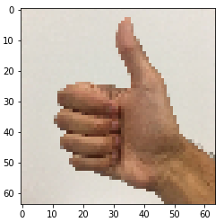
fname = "images/thumbs_up.jpg"
image = np.array(ndimage.imread(fname, flatten=False))
my_image = scipy.misc.imresize(image, size=(64,64))
plt.imshow(my_image)