Emotion Recognition Using Graph Convolutional Networks
2019-10-22 09:26:56
This blog is from: https://towardsdatascience.com/emotion-recognition-using-graph-convolutional-networks-9f22f04b244e
Recently, deep learning has made much progress in natural language processing (NLP). With many new inventions such as Attention and Transformers leading to state of the art models such as BERT and XLNet, many tasks such as textual emotion recognition have become easier. This article will introduce a new method to conduct emotion recognition from conversations using graphs.
What is Emotion Recognition?
Simply put, emotion recognition (ERC) is the task of classifying the emotion behind a piece of written task. Given a piece of text can you tell if the speaker is angry, happy, sad, or perhaps confused? It has many far-ranging applications in healthcare, education, sales, and human resources. At the highest level, the task of ERC is useful because many are convinced that it is a stepping stone to building a conversationally intelligent AI that is able to talk with a human.

Currently, the two major pieces of innovation that most ERC is built on are recurrent neural networks (RNN) and attention mechanisms. RNNs such as LSTMs and GRUs look at text sequentially. When the text is long, the model’s memory of the beginning parts is lost. Attention mechanisms solve this well by weighing different parts of the sentence differently.
However, RNNs+Attention still have trouble taking into context of personality, topic, and intent from neighboring sequences and also the speaker (basically all the very important parts of any conversation). Couple this with the lack of labeled benchmark datasets for personality/emotion it becomes really difficult not just to implement but also to measure the result of new models. This article will summarize a recent paper that solves much of this by using a relatively new innovation called graph convolution networks: DialogueGCN: A Graph Convolutional Neural Network for Emotion Recognition in Conversation [1].
Context Matters
In a conversation, context matters. A simple “Okay” can mean “Okay?”, “Okay!” or “Okay….” depending on what you and the other said before, how you are feeling, how the other person is feeling, the level of tension and many other things. There are two types of context that matter:
- Sequential Context: The meaning of a sentence in a sequence. This context deals with how past words impact future words, the relationship of words, and semantic/syntactic features. Sequential context is taken into account in RNN models with attention.
- Speaker Level Context: Inter and intra-speaker dependency. This context deals with the relation between the speakers as well as self-dependency: the notion that your own personality change and affect how you speak during the course of the conversation.
As you can probably guess, it’s speaker level context that most models have difficulty taking into account. It turns out you can actually model speaker level context very well using graph convolutional neural networks and this is exactly the approach DialogueGCN takes.
Representing Conversations as Graphs
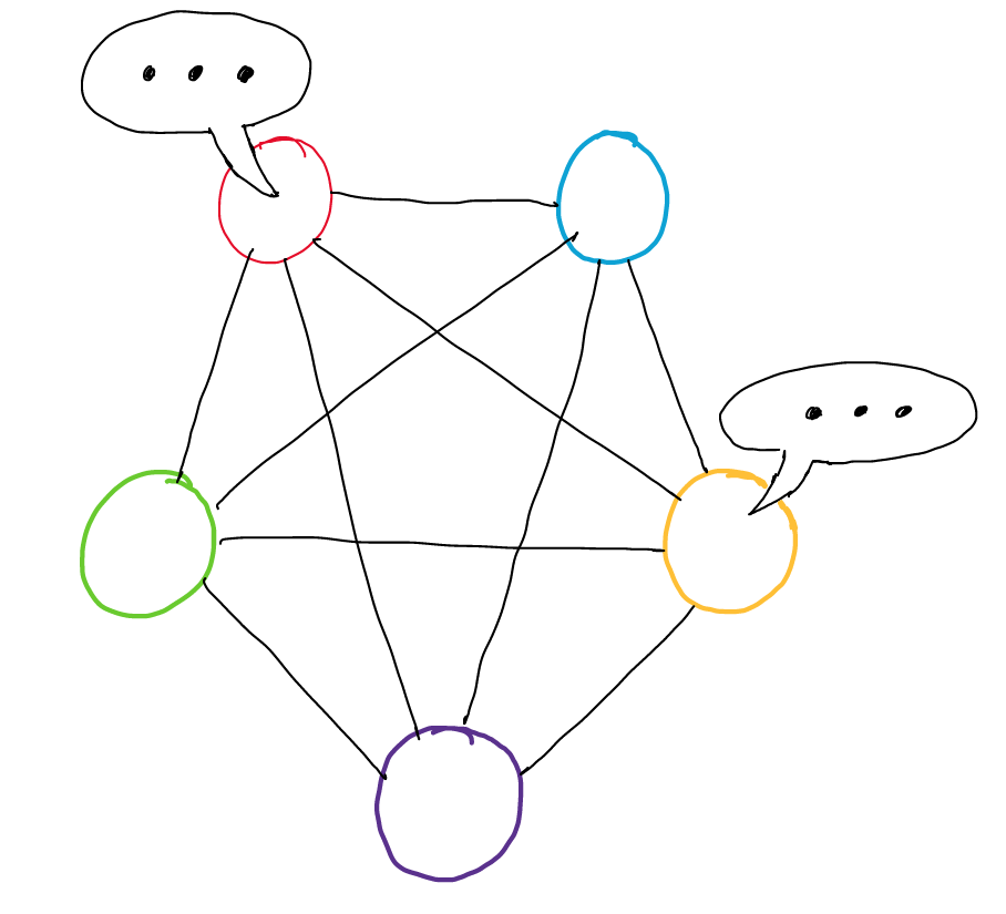
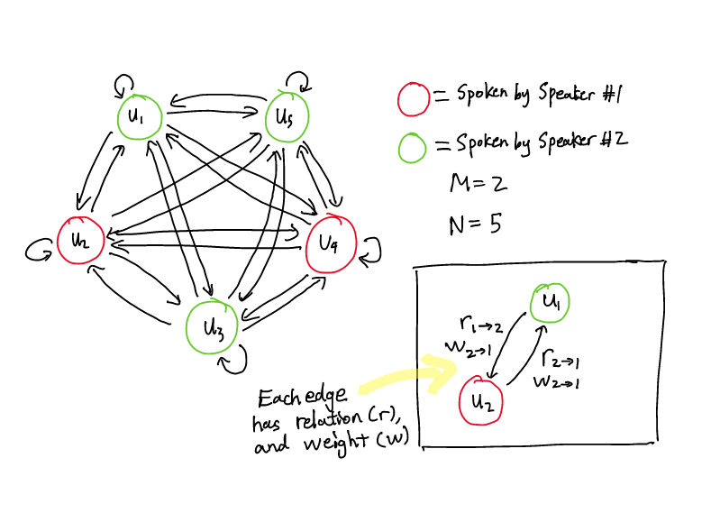
In a conversation there are M speakers/parties represented as p[1], p[2], . . . , p[M]. Each utterance (a piece of text someone sends) is represented as u[1], u[2], . . . , u[N]. The final goal in ERC is to accurately predict each utterance as one of happy, sad, neutral, angry, excited, frustrated, disgust, or fear.

The entire conversation can be built as a directed graph:
G = (V, E, R, W)
- Utterances are the nodes (V). Edges are paths/connections between the nodes (E). Relations are the different types/labels of the edges (R). Weights represent the importance of an edge (W).
- Every edge between two nodes v[i] and v[j] has two properties: the relation (r) and weight (w). We’ll talk more about this in just a bit.
- The graph is directed. Therefore, all edges are one way. The edge from v[i] to v[j] is different from the edge that goes from v[j] to v[i].
One thing to notice from the figure is that each utterance has an edge connected to itself. This represents the relation of the utterance to itself. In more practical terms, this is how an utterance impacts the mind of the utterance’s speaker.
Context Window
One major problem of a graph representation is that if a conversation is really long, there can be many edges for a single node. And since each node is connected to every other node, it scales quadratically as the size of the graph increases. This is very computationally expensive.
To resolve this problem, in DialogueGCN, the graph’s edges are constructed based on a context window with a specific size. So for a node/utterance i, only the past size and future size utterances are connected in a graph (any node in the range of i-size to i+size).

Edge Weights
Edge weight are calculated using an attention function. The attention function is set up so that for each node/utterance, the incoming edge weights all sum up to 1. Edge weights are constant and do not change in the learning process.
In simplified terms, the edge weight represents the importance of the connection between two nodes.
Relations
The relation of an edge depends on two things:
- Speaker dependency: Who spoke u[i]? Who spoke v[j]?
- Temporal dependency: Was u[i] uttered before u[j], or the other way around?
In a conversation, if there are M different speakers, there will be a maximum of M (speaker of u[j]) * M (speaker of u[j]) * 2 (whether u[i] occurs before u[j], or the reverse) = 2M² relations.
We can list all of the relations from our example graph above:
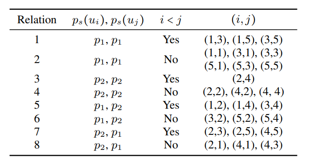
Here’s the same graph with the edges’ relation labelled according to the table:

In our example, we have 8 different relation. At a high level, relation is an important property for the edge because who spoke what and when matters a lot in a conversation. If Peter asks a question and Jenny responds, this is different from Jenny first saying the answer and then Peter asking the question (temporal dependency). Likewise, if Peter asks the same question to Jenny and Bob, they may respond differently (speaker dependency).
Think of the relation as defining the type of the connection, and the edge weight representing the importance of the connection.
Think of the relation as defining the type of the connection, and the edge weight representing the importance of the connection.
The Model
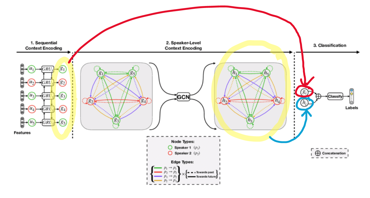
The DialogueGCN model uses a type of graph neural network known as a graph convolutional network (GCN).
Just like above, the example shown is for a 2 speaker 5 utterance graph.

In stage 1, each utterance u[i] is represented as a feature vector and given sequential context encoding. This is done by running each utterance through a series of GRUs in a sequential context encoder. A graph structure is not needed for stage 1. The new utterance with sequential context is denoted as g[1]……. g[N] in the paper. This is the input to the GCN.

In stage 2, the model constructs a graph like discussed in the previous section and will add speaker level context to the graph using feature transformation. The utterances with BOTH sequential and speaker level context is denoted by h[1]……h[N]. This is the output of the GCN.
The difference in the looks of the edges and nodes (dash vs solid, different colors) represents a different relation. For example, green g[1] to green g[3], with a solid green edge is relation 1 in the table.
Feature Transformation — Embedding Speaker Level Context
One of the most important steps of the GCN is feature transformation — basically how the GCN will embed speaker level context into the utterances. We will first discuss the technique used and then describe where the intuition for it came from.
There are two steps in a feature transformation. In step 1, for each node h[i] neighboring node information (nodes within the context window size) is aggregated to create a new feature vector h[i]¹.

The function might look complicated but at its core just think of it as a layer in the network with learnable parameters denoted by W[0]¹ and W[r]¹. One thing that was added is a constant c[i,r] which is a normalization constant. It can be set in advance or learned with the network itself.
As mentioned before, edge weights are constant and are not changed or learned in the process.
In step 2, the same thing is basically done again. Neighbor information is aggregated and a similar function is applied to the output of step 1.

Once again, W² and W[0]² represent learnable parameters that are modified in the training process.
At a high level, this two step process essentially takes a normalized sum of all the neighboring utterance information for each utterance. At a deeper level, this two step transformation has its root in what’s known as a simple differentiable message-passing framework [2]. This technique was taken by researchers working on graph convolutional neural networks to model relational data [3]. If you have time, I would highly recommend giving those two papers a read in that order. I believe all the intuition needed for DialogueGCN’s feature transformation process is in those two papers.
The output of the GCN is denoted by h[1]…..h[N] on the figure.
In stage 3, the original sequential context encoded vectors are concatenated with the speaker level context encoded vectors. This is similar to combining original layers with later layers to “summarize” the outputs of every layer.
The concatenated feature vector is then fed into a fully connected network for classification. The final output is a probability distribution of the different emotions the model thinks the utterance is.
The training of the model is done using a categorical-cross-entropy loss with L2-regularization. This loss is used because the model is predicting the probability of multiple labels (emotion classes).
Results
Benchmark Datasets
Previously we mentioned the lack of benchmark datasets. The authors of the paper were able to solve this by using labeled multimodal datasets (text along with video or audio) and then extracting the textual portion and completely ignoring any audio or visual data.
DialogueGCN was evaluated on these datasets:
- IEMOCAP: Two-way conversations of ten unique speakers in video format. Utterances are labeled with either happy, sad, neutral, angry, excited, or frustrated.
- AVEC: Conversations between humans and artificially intelligent agents. Utterances have four labels: valence ([-1,1]), arousal ([-1, 1]), expectancy ([-1,1]), and power ([0, infinity]).
- MELD: Contains 1400 dialogues and 13000 utterances from the TV series Friends. MELD also contains complementary acoustic and visual information. Utterances are labeled as one of anger, disgust, sadness, joy, surprise, fear, or neutral.
MELD has a pre-defined train/validation/test split. AVEC and IEMOCAP do not have predefined splits so 10% of the dialogues were used as the validation set.
DialogueGCN was compared to many baseline and state of the art models for ERC. One particular state of the art model was DialogueRNN by the same authors of the paper.
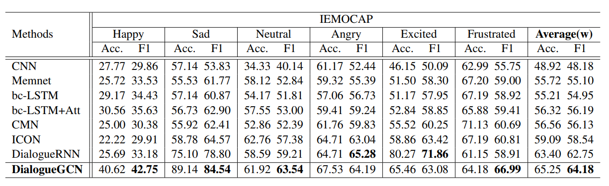
In 4 of the 6 categories of IEMOCAP, DialogueGCN shows a noticeable improvement against all models including DialogueRNN. In the “Angry” category, DialogueGCN essentially ties with DialogueRNN (GCN is only worse by 1.09 on the F1 score). Only the “Excited” category shows a large enough difference.
DialogueGCN is able to produce similar results on AVEC and MELD, beating out the incumbent DialogueRNN.

What is clear from the result is that adding speaker level context to a conversation graph inherently improves understanding. DialogueRNN, which captured sequential context well, lacked the ability to encode speaker context.
Analysis
One parameter that was experimented with is the size of the context window. By extending the size, one is able to increase the number of edges to a specific utterance. It was found that an increase in the size, while more computationally expensive, improved results.
Another interesting experiment the authors did was an ablation study. The encoders were removed one at a time and the performance was re-measured. It was found that the speaker-level context encoder (stage 2) was slightly more important than the sequential context encoder (stage 1).
It was also found that misclassification tended to happen among two scenarios:
- Similar emotion classes such as “frustrated” and “angry”, or “excited” and “happy”.
- Short utterances such as “okay” or “yeah”.
Because all the datasets used were multimodal and contained audio and video, it’s possible to improve the accuracy within these two scenarios by integrating audio and visual multimodal learning. And while misclassification still happens, it’s important to note that DialogueGCN still resulted in a very noticeable improvement in accuracy.
Key Takeaways
- Context matters. A good model will not only take into account the sequential context of the conversation (order of sentences, which words relate to the other), but also the speaker level context (who says what, when they are saying it, how they are impacted by other speakers and themselves). Integrating speaker level context is a big step forward from the traditional sequential and attention-based models.
- Sequences aren’t the only way you can represent conversations. If there’s one thing this paper shows, it’s that the structure of the data can help capture a lot of context. In this case, speaker level context was much more easily encoded in a graph format.
- Graph neural networks are a promising avenue of research in NLP. The key concept of aggregating the information of neighbors, while simple conceptually, is amazingly powerful at capturing relationships in data.
Thanks for reading!
You can connect with me on Medium, Linkedin, or [email protected]
Original Paper: https://arxiv.org/abs/1908.11540
Sources:
[1] Ghosal, Deepanway & Majumder, Navonil & Poria, Soujanya & Chhaya, Niyati & Gelbukh, Alexander. (2019). DialogueGCN: A Graph Convolutional Neural Network for Emotion Recognition in Conversation.
[2] Michael Schlichtkrull, Thomas N Kipf, Peter Bloem, Rianne Van Den Berg, Ivan Titov, and Max Welling. 2018. Modeling relational data with graph convolutional networks. In European Semantic Web Conference, pages 593–607. Springer.
[3] Justin Gilmer, Samuel S Schoenholz, Patrick F Riley, Oriol Vinyals, and George E Dahl. 2017. Neural message passing for quantum chemistry. In Proceedings of the 34th International Conference on Machine Learning-Volume 70, pages 1263–1272. JMLR. org.