本文通过利用信用卡的历史交易数据进行机器学习，构建信用卡反欺诈预测模型，对客户信用卡盗刷进行预测

一、项目背景

对信用卡盗刷事情进行预测对于挽救客户、银行损失意义十分重大，此项目数据集来源于Kaggle，数据集包含由欧洲持卡人于2013年9月使用信用卡进行交的数据。此数据集显示两天内发生的交易，其中284,807笔交易中有492笔被盗刷。数据集非常不平衡，积极的类（被盗刷）占所有交易的0.172％。因判定信用卡持卡人信用卡是否会被盗刷为二分类问题，解决分类问题我们可以有逻辑回归、SVM、随机森林算法，也可利用boost集成学习的XGboost算法进行数据的训练与判别，本文中采用逻辑回归算法进行测试。

二、探索性数据分析

2.1 理解数据

import numpy as np
import pandas as pd

data = pd.read_csv('E:\\数据挖掘\\Project\\信用卡反欺诈模型\\creditcardfraud\\creditcard.csv')
len(data)
data.info()
data.head()

Data columns (total 31 columns):
Time      284807 non-null float64
V1        284807 non-null float64
V2        284807 non-null float64
V3        284807 non-null float64
V4        284807 non-null float64
V5        284807 non-null float64
V6        284807 non-null float64
V7        284807 non-null float64
V8        284807 non-null float64
V9        284807 non-null float64
V10       284807 non-null float64
V11       284807 non-null float64
V12       284807 non-null float64
V13       284807 non-null float64
V14       284807 non-null float64
V15       284807 non-null float64
V16       284807 non-null float64
V17       284807 non-null float64
V18       284807 non-null float64
V19       284807 non-null float64
V20       284807 non-null float64
V21       284807 non-null float64
V22       284807 non-null float64
V23       284807 non-null float64
V24       284807 non-null float64
V25       284807 non-null float64
V26       284807 non-null float64
V27       284807 non-null float64
V28       284807 non-null float64
Amount    284807 non-null float64
Class     284807 non-null int64
dtypes: float64(30), int64(1)

Time        V1        V2        V3  ...       V27       V28  Amount  Class
0   0.0 -1.359807 -0.072781  2.536347  ...  0.133558 -0.021053  149.62      0
1   0.0  1.191857  0.266151  0.166480  ... -0.008983  0.014724    2.69      0
2   1.0 -1.358354 -1.340163  1.773209  ... -0.055353 -0.059752  378.66      0
3   1.0 -0.966272 -0.185226  1.792993  ...  0.062723  0.061458  123.50      0
4   2.0 -1.158233  0.877737  1.548718  ...  0.219422  0.215153   69.99      0

可见数据共有31列，284807行，其中V1-V28为结构化数据，另一列为整形数据，也为类别属性Class，Amount和Time的数据特征与规格与其他特征不大相同，此外还显示了各列的均值、最小值、最大值、四分位数

2.2 数据初步探索

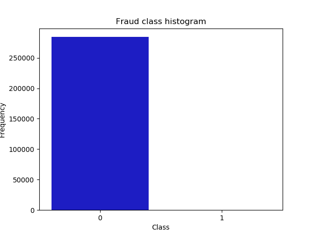
No Frauds 99.83 % of the dataset
Frauds 0.17 % of the dataset

可以看出数据很不均衡：数据不均衡很可能导致我们模型预测结果‘0’时很准确，而预测‘1’时并不准确。

2.3 数据预处理

由上图知Fraud 与No Fraud的数据不均衡，若直接进行数据建模则会造成如下问题：

1）过拟合，因样本中存在大量的正例（No Fraud），故机器可能过多学习正例的特征而造成判断错误

2）特征关联错误，因样本数据不平衡，容易将不同的特征属性误关联

解决方案有如下：

1）Random undersampling，欠采样

通过选取正例中与Fraud相同数量的样本构成均衡的样本，这样新的样本样本中，Fraud、No Fraud各占50%

2）Oversampling，过采样

采用SMOTE算法，从少数类Fraud中创建合成点，以便在少数类和多数类之间达到平衡，不必删除任何行，这与随机欠采样不同，也由于没有如前所述未删除任何行，因此需要更多时间进行训练

需要说明的是虽然我们在实现Random Undersampling或Oversampling技术时对数据进行处理，但仍需要原始测试集上测试我们的模型，而不是在欠采样或过采样上。欠采样和过采样的作用是使构建的模型合适，最终还是服务于原始数据集。之后对分别采用欠采样和过采样的方法进行数据处理、建模，再对原始数据集进行预测分析。

此外还发现Amount列数值较大，不符合数据相似性原则，因此需要归一化使其范围在（-1， 1），否则在进行皮尔逊相关性分析时会出错。

三、特征工程

1. 绘制各种特征的分布图

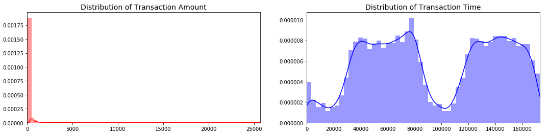
1 ）查看盗刷与正常刷卡的刷卡金额分布图

\(信用卡被盗刷发生的金额与信用卡正常用户发生的金额相比，比较小。这说明信用卡盗刷者为了不引起信用卡卡主的注意，更偏向选择小金额消费\)

2）查看交易时间与交易金额的分布图

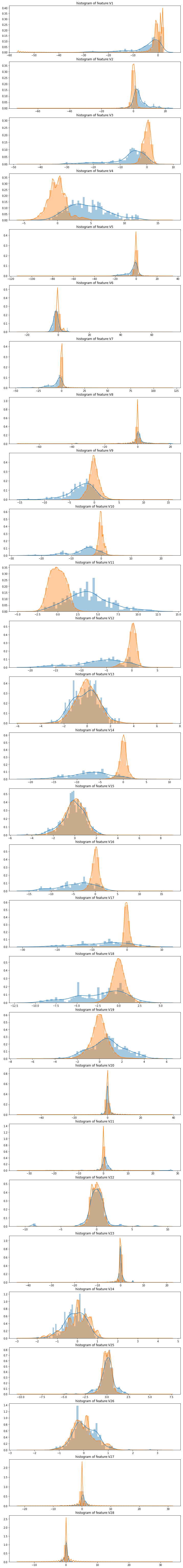
3）查看其他特征的分布图

2. 处理不平衡数据

对Amount进行归一化，使其范围在（-1， 1）

from sklearn.preprocessing import StandardScaler

data['normAmount'] = StandardScaler().fit_transform(data['Amount'].reshape(-1, 1))
data = data.drop(['Time','Amount'],axis=1)
data.head()

此外还需要进行采用处理，分为欠采样处理和过采样处理，Random undersampling 和 Oversampling，这里先按照欠处理采样进行分析。因此我们得到一个正反例平衡的数据样本。

X = data.ix[:,data.columns != 'Class']
Y = data.ix[:,data.columns == 'Class']

number_record_fraud = len(Y[Y.Class==1])

fraud_indices = np.array(data[data.Class == 1].index)
normal_indices = np.array(data[data.Class == 0].index)
random_normal_indices = np.array(np.random.choice(normal_indices,number_record_fraud,replace=False))

under_sample_indices = np.concatenate([fraud_indices,random_normal_indices])
under_sample_data = data.iloc[under_sample_indices,:]

X_under_sample = under_sample_data.ix[:,under_sample_data.columns != 'Class']
Y_under_sample = under_sample_data.ix[:,under_sample_data.columns == 'Class']

from sklearn.cross_validation import train_test_split

X_train_under_sample,X_test_under_sample,Y_train_under_sample,Y_test_under_sample = train_test_split(X_under_sample,Y_under_sample,test_size=0.3,random_state=0)

X_train, X_test, Y_train, Y_test = train_test_split(X, Y, test_size=0.3, random_state=0)

3.相关性特征分析

3.1 相关性分析

f, (ax1, ax2) = plt.subplots(2, 1, figsize=(24,20))

sub_sample_corr = new_df.corr()
sns.heatmap(sub_sample_corr, cmap='coolwarm_r', annot_kws={'size':20}, ax=ax2)
ax2.set_title('SubSample Correlation Matrix \n', fontsize=14)
plt.show()

avatar

通过heatmap发现， V17，V14，V12和V10呈负相关，这意味着这些值越低，最终结果就越有可能成为欺诈交易，V4，V11和V19正相关。注意这些值越高，最终结果越有可能成为欺诈交易。

3.2 箱线图

绘制上述的正相关、负相关的特征属性的箱线图

f, axes = plt.subplots(ncols=4, figsize=(20,4))

# Negative Correlations with our Class (The lower our feature value the more likely it will be a fraud transaction)
sns.boxplot(x="Class", y="V17", data=new_df, palette=colors, ax=axes[0])
axes[0].set_title('V17 vs Class Negative Correlation')

sns.boxplot(x="Class", y="V14", data=new_df, palette=colors, ax=axes[1])
axes[1].set_title('V14 vs Class Negative Correlation')


sns.boxplot(x="Class", y="V12", data=new_df, palette=colors, ax=axes[2])
axes[2].set_title('V12 vs Class Negative Correlation')


sns.boxplot(x="Class", y="V10", data=new_df, palette=colors, ax=axes[3])
axes[3].set_title('V10 vs Class Negative Correlation')

plt.show()

avatar

f, axes = plt.subplots(ncols=4, figsize=(20,4))

# Positive correlations (The higher the feature the probability increases that it will be a fraud transaction)
sns.boxplot(x="Class", y="V11", data=new_df, palette=colors, ax=axes[0])
axes[0].set_title('V11 vs Class Positive Correlation')

sns.boxplot(x="Class", y="V4", data=new_df, palette=colors, ax=axes[1])
axes[1].set_title('V4 vs Class Positive Correlation')


sns.boxplot(x="Class", y="V2", data=new_df, palette=colors, ax=axes[2])
axes[2].set_title('V2 vs Class Positive Correlation')


sns.boxplot(x="Class", y="V19", data=new_df, palette=colors, ax=axes[3])
axes[3].set_title('V19 vs Class Positive Correlation')

plt.show()

avatar

3.3 异常值处理

在异常值处理前，需要可视化我们将要使用的特征的。由于上述V17、V14、V12、V10为负相关特征，观察这些特征的分布，与其他相比，V14是唯一具有高斯分布的特征。根据四分位数确定阀值，对在阀值外的异常数据进行剔除。

from scipy.stats import norm

f, (ax1, ax2, ax3) = plt.subplots(1,3, figsize=(20, 6))

v14_fraud_dist = new_df['V14'].loc[new_df['Class'] == 1].values
sns.distplot(v14_fraud_dist,ax=ax1, fit=norm, color='#FB8861')
ax1.set_title('V14 Distribution \n (Fraud Transactions)', fontsize=14)

v12_fraud_dist = new_df['V12'].loc[new_df['Class'] == 1].values
sns.distplot(v12_fraud_dist,ax=ax2, fit=norm, color='#56F9BB')
ax2.set_title('V12 Distribution \n (Fraud Transactions)', fontsize=14)


v10_fraud_dist = new_df['V10'].loc[new_df['Class'] == 1].values
sns.distplot(v10_fraud_dist,ax=ax3, fit=norm, color='#C5B3F9')
ax3.set_title('V10 Distribution \n (Fraud Transactions)', fontsize=14)

plt.show()

avatar

# # -----> V14 Removing Outliers (Highest Negative Correlated with Labels)
v14_fraud = new_df['V14'].loc[new_df['Class'] == 1].values
q25, q75 = np.percentile(v14_fraud, 25), np.percentile(v14_fraud, 75)
print('Quartile 25: {} | Quartile 75: {}'.format(q25, q75))
v14_iqr = q75 - q25
print('iqr: {}'.format(v14_iqr))

v14_cut_off = v14_iqr * 1.5
v14_lower, v14_upper = q25 - v14_cut_off, q75 + v14_cut_off
print('Cut Off: {}'.format(v14_cut_off))
print('V14 Lower: {}'.format(v14_lower))
print('V14 Upper: {}'.format(v14_upper))

outliers = [x for x in v14_fraud if x < v14_lower or x > v14_upper]
print('Feature V14 Outliers for Fraud Cases: {}'.format(len(outliers)))
print('V10 outliers:{}'.format(outliers))

new_df = new_df.drop(new_df[(new_df['V14'] > v14_upper) | (new_df['V14'] < v14_lower)].index)
print('----' * 44)

# -----> V12 removing outliers from fraud transactions
v12_fraud = new_df['V12'].loc[new_df['Class'] == 1].values
q25, q75 = np.percentile(v12_fraud, 25), np.percentile(v12_fraud, 75)
v12_iqr = q75 - q25

v12_cut_off = v12_iqr * 1.5
v12_lower, v12_upper = q25 - v12_cut_off, q75 + v12_cut_off
print('V12 Lower: {}'.format(v12_lower))
print('V12 Upper: {}'.format(v12_upper))
outliers = [x for x in v12_fraud if x < v12_lower or x > v12_upper]
print('V12 outliers: {}'.format(outliers))
print('Feature V12 Outliers for Fraud Cases: {}'.format(len(outliers)))
new_df = new_df.drop(new_df[(new_df['V12'] > v12_upper) | (new_df['V12'] < v12_lower)].index)
print('Number of Instances after outliers removal: {}'.format(len(new_df)))
print('----' * 44)


# Removing outliers V10 Feature
v10_fraud = new_df['V10'].loc[new_df['Class'] == 1].values
q25, q75 = np.percentile(v10_fraud, 25), np.percentile(v10_fraud, 75)
v10_iqr = q75 - q25

v10_cut_off = v10_iqr * 1.5
v10_lower, v10_upper = q25 - v10_cut_off, q75 + v10_cut_off
print('V10 Lower: {}'.format(v10_lower))
print('V10 Upper: {}'.format(v10_upper))
outliers = [x for x in v10_fraud if x < v10_lower or x > v10_upper]
print('V10 outliers: {}'.format(outliers))
print('Feature V10 Outliers for Fraud Cases: {}'.format(len(outliers)))
new_df = new_df.drop(new_df[(new_df['V10'] > v10_upper) | (new_df['V10'] < v10_lower)].index)
print('Number of Instances after outliers removal: {}'.format(len(new_df)))

f,(ax1, ax2, ax3) = plt.subplots(1, 3, figsize=(20,6))

colors = ['#B3F9C5', '#f9c5b3']
# Boxplots with outliers removed
# Feature V14
sns.boxplot(x="Class", y="V14", data=new_df,ax=ax1, palette=colors)
ax1.set_title("V14 Feature \n Reduction of outliers", fontsize=14)
ax1.annotate('Fewer extreme \n outliers', xy=(0.98, -17.5), xytext=(0, -12),
            arrowprops=dict(facecolor='black'),
            fontsize=14)

# Feature 12
sns.boxplot(x="Class", y="V12", data=new_df, ax=ax2, palette=colors)
ax2.set_title("V12 Feature \n Reduction of outliers", fontsize=14)
ax2.annotate('Fewer extreme \n outliers', xy=(0.98, -17.3), xytext=(0, -12),
            arrowprops=dict(facecolor='black'),
            fontsize=14)

# Feature V10
sns.boxplot(x="Class", y="V10", data=new_df, ax=ax3, palette=colors)
ax3.set_title("V10 Feature \n Reduction of outliers", fontsize=14)
ax3.annotate('Fewer extreme \n outliers', xy=(0.95, -16.5), xytext=(0, -12),
            arrowprops=dict(facecolor='black'),
            fontsize=14)


plt.show()

avatar

3.3 降维

降维的作用是将高维的数据集中不必要的特征去除，只保留需要的特征属性。

f, (ax1, ax2, ax3) = plt.subplots(1, 3, figsize=(24,6))
# labels = ['No Fraud', 'Fraud']
f.suptitle('Clusters using Dimensionality Reduction', fontsize=14)


blue_patch = mpatches.Patch(color='#0A0AFF', label='No Fraud')
red_patch = mpatches.Patch(color='#AF0000', label='Fraud')


# t-SNE scatter plot
ax1.scatter(X_reduced_tsne[:,0], X_reduced_tsne[:,1], c=(y == 0), cmap='coolwarm', label='No Fraud', linewidths=2)
ax1.scatter(X_reduced_tsne[:,0], X_reduced_tsne[:,1], c=(y == 1), cmap='coolwarm', label='Fraud', linewidths=2)
ax1.set_title('t-SNE', fontsize=14)

ax1.grid(True)

ax1.legend(handles=[blue_patch, red_patch])


# PCA scatter plot
ax2.scatter(X_reduced_pca[:,0], X_reduced_pca[:,1], c=(y == 0), cmap='coolwarm', label='No Fraud', linewidths=2)
ax2.scatter(X_reduced_pca[:,0], X_reduced_pca[:,1], c=(y == 1), cmap='coolwarm', label='Fraud', linewidths=2)
ax2.set_title('PCA', fontsize=14)

ax2.grid(True)

ax2.legend(handles=[blue_patch, red_patch])

# TruncatedSVD scatter plot
ax3.scatter(X_reduced_svd[:,0], X_reduced_svd[:,1], c=(y == 0), cmap='coolwarm', label='No Fraud', linewidths=2)
ax3.scatter(X_reduced_svd[:,0], X_reduced_svd[:,1], c=(y == 1), cmap='coolwarm', label='Fraud', linewidths=2)
ax3.set_title('Truncated SVD', fontsize=14)

ax3.grid(True)

ax3.legend(handles=[blue_patch, red_patch])

plt.show()

avatar

四、数据建模与评估

4.1 Recall

引入recall，针对上述Random undersampling 欠采样，进行LR回归训练

#Recall = TP/(TP+FN)
from sklearn.linear_model import LogisticRegression
from sklearn.cross_validation import KFold, cross_val_score
from sklearn.metrics import confusion_matrix,recall_score,classification_report

4.2 Logistic Regression

def printing_Kfold_scores(x_train_data,y_train_data):
    fold = KFold(len(y_train_data),5,shuffle=False) 

    # Different C parameters
    c_param_range = [0.01,0.1,1,10,100]

    results_table = pd.DataFrame(index = range(len(c_param_range),2), columns = ['C_parameter','Mean recall score'])
    results_table['C_parameter'] = c_param_range

    # the k-fold will give 2 lists: train_indices = indices[0], test_indices = indices[1]
    j = 0
    for c_param in c_param_range:
        print('-------------------------------------------')
        print('C parameter: ', c_param)
        print('-------------------------------------------')
        print('')

        recall_accs = []
        for iteration, indices in enumerate(fold,start=1):

            # Call the logistic regression model with a certain C parameter
            lr = LogisticRegression(C = c_param, penalty = 'l1')

            # Use the training data to fit the model. In this case, we use the portion of the fold to train the model
            # with indices[0]. We then predict on the portion assigned as the 'test cross validation' with indices[1]
            lr.fit(x_train_data.iloc[indices[0],:],y_train_data.iloc[indices[0],:].values.ravel())

            # Predict values using the test indices in the training data
            y_pred_undersample = lr.predict(x_train_data.iloc[indices[1],:].values)

            # Calculate the recall score and append it to a list for recall scores representing the current c_parameter
            recall_acc = recall_score(y_train_data.iloc[indices[1],:].values,y_pred_undersample)
            recall_accs.append(recall_acc)
            print('Iteration ', iteration,': recall score = ', recall_acc)

        # The mean value of those recall scores is the metric we want to save and get hold of.
        results_table.ix[j,'Mean recall score'] = np.mean(recall_accs)
        j += 1
        print('')
        print('Mean recall score ', np.mean(recall_accs))
        print('')

    best_c = results_table.loc[results_table['Mean recall score'].idxmax()]['C_parameter']
    
    # Finally, we can check which C parameter is the best amongst the chosen.
    print('*********************************************************************************')
    print('Best model to choose from cross validation is with C parameter = ', best_c)
    print('*********************************************************************************')
    
    return best_c

4.3 混淆矩阵

因单一使用recall值来评价模型还是有一定的缺陷，现引入混淆矩阵来进一步对模型进行评估。

import itertools
def plot_confusion_matrix(cm, classes,
                          title='Confusion matrix',
                          cmap=plt.cm.Blues):
    """
    This function prints and plots the confusion matrix.
    """
    plt.imshow(cm, interpolation='nearest', cmap=cmap)
    plt.title(title)
    plt.colorbar()
    tick_marks = np.arange(len(classes))
    plt.xticks(tick_marks, classes, rotation=0)
    plt.yticks(tick_marks, classes)

    thresh = cm.max() / 2.
    for i, j in itertools.product(range(cm.shape[0]), range(cm.shape[1])):
        plt.text(j, i, cm[i, j],
                 horizontalalignment="center",
                 color="white" if cm[i, j] > thresh else "black")

    plt.tight_layout()
    plt.ylabel('True label')
    plt.xlabel('Predicted label')

lr = LogisticRegression(C = best_c, penalty = 'l1')
y_pred_undersample_score = lr.fit(X_train_undersample,y_train_undersample.values.ravel()).decision_function(X_test_undersample.values)
fpr, tpr, thresholds = roc_curve(y_test_undersample.values.ravel(),y_pred_undersample_score)
roc_auc = auc(fpr,tpr)
# Plot ROC
plt.title('Receiver Operating Characteristic')
plt.plot(fpr, tpr, 'b',label='AUC = %0.2f'% roc_auc)
plt.legend(loc='lower right')
plt.plot([0,1],[0,1],'r--')
plt.xlim([-0.1,1.0])
plt.ylim([-0.1,1.01])
plt.ylabel('True Positive Rate')
plt.xlabel('False Positive Rate')
plt.show()

best_c = printing_Kfold_scores(X_train,y_train)
lr = LogisticRegression(C = best_c, penalty = 'l1')
lr.fit(X_train,y_train.values.ravel())
y_pred_undersample = lr.predict(X_test.values)
cnf_matrix = confusion_matrix(y_test,y_pred_undersample)
np.set_printoptions(precision=2)
print("Recall metric in the testing dataset: ", cnf_matrix[1,1]/(cnf_matrix[1,0]+cnf_matrix[1,1]))
 
class_names = [0,1]
plt.figure()
plot_confusion_matrix(cnf_matrix
                      , classes=class_names
                      , title='Confusion matrix')
plt.show()
lr = LogisticRegression(C = best_c, penalty = 'l1')
y_pred_score = lr.fit(X_train,y_train.values.ravel()).decision_function(X_test.values)
fpr, tpr, thresholds = roc_curve(y_test.values.ravel(),y_pred_score)
roc_auc = auc(fpr,tpr)
 
plt.title('Receiver Operating Characteristic')
plt.plot(fpr, tpr, 'b',label='AUC = %0.2f'% roc_auc)
plt.legend(loc='lower right')
plt.plot([0,1],[0,1],'r--')
plt.xlim([-0.1,1.0])
plt.ylim([-0.1,1.01])
plt.ylabel('True Positive Rate')
plt.xlabel('False Positive Rate')
plt.show()

4.4 原始数据分析

上面是用下采样处理得到的测试数据来求recall和混淆矩阵的，因为下采样得到的数据相比于原始数据是很少的，所以这个测试结果没什么说服力，所以我们要用原始数据（没有经过下采样的数据）来进行测试

lr = LogisticRegression(C = best_c, penalty = 'l1')
lr.fit(X_train_under_sample,Y_train_under_sample.values.ravel())
Y_pred = lr.predict(X_test.values)

# Compute confusion matrix
cnf_matrix = confusion_matrix(Y_test,Y_pred)
np.set_printoptions(precision=2)

print("Recall metric in the testing dataset: ", float(cnf_matrix[1,1])/(cnf_matrix[1,0]+cnf_matrix[1,1]))

# Plot non-normalized confusion matrix
class_names = [0,1]
plt.figure()
plot_confusion_matrix(cnf_matrix
                      , classes=class_names
                      , title='Confusion matrix')
plt.show()

逻辑回归模型中除了惩罚力度参数C需要整定，Threshold也可以调调，默认不做处理相当于Threshold为0.5



lr = LogisticRegression(C = 0.01, penalty = 'l1')
lr.fit(X_train_undersample,y_train_undersample.values.ravel())
y_pred_undersample_proba = lr.predict_proba(X_test_undersample.values)

thresholds = [0.1,0.2,0.3,0.4,0.5,0.6,0.7,0.8,0.9]

plt.figure(figsize=(10,10))

j = 1
for i in thresholds:
    y_test_predictions_high_recall = y_pred_undersample_proba[:,1] > i
    
    plt.subplot(3,3,j)
    j += 1
    
    # Compute confusion matrix
    cnf_matrix = confusion_matrix(y_test_undersample,y_test_predictions_high_recall)
    np.set_printoptions(precision=2)

    print("Recall metric in the testing dataset: ", cnf_matrix[1,1]/(cnf_matrix[1,0]+cnf_matrix[1,1]))

    # Plot non-normalized confusion matrix
    class_names = [0,1]
    plot_confusion_matrix(cnf_matrix
                          , classes=class_names
                          , title='Threshold >= %s'%i)

4.5 过采样处理

现在使用SMOTE过采样进行分析

import numpy as np
import pandas as pd
import matplotlib.pyplot as plt

from imblearn.over_sampling import SMOTE
from sklearn.ensemble import RandomForestClassifier
from sklearn.metrics import confusion_matrix
from sklearn.model_selection import train_test_split

data = pd.read_csv('creditcard.csv')

from sklearn.preprocessing import StandardScaler
data['normAmount'] = StandardScaler().fit_transform(data['Amount'].values.reshape(-1,1)) 

data = data.drop(['Amount','Time'], axis=1)

import itertools
from sklearn.linear_model import LogisticRegression
from sklearn.cross_validation import KFold, cross_val_score
from sklearn.metrics import confusion_matrix,recall_score,classification_report 

def printing_Kfold_scores(x_train_data,y_train_data):
    fold = KFold(len(y_train_data),5,shuffle=False) 

    c_param_range = [0.01,0.1,1,10,100]

    results_table = pd.DataFrame(index = range(len(c_param_range),2), columns = ['C_parameter','Mean recall score'])
    results_table['C_parameter'] = c_param_range

    j = 0
    for c_param in c_param_range:
        print('-------------------------------------------')
        print('C parameter: ', c_param)
        print('-------------------------------------------')
        print('')

        recall_accs = []
        for iteration, indices in enumerate(fold,start=1):
            lr = LogisticRegression(C = c_param, penalty = 'l1')
lr.fit(x_train_data.iloc[indices[0],:],y_train_data.iloc[indices[0],:].values.ravel())
            y_pred_undersample = lr.predict(x_train_data.iloc[indices[1],:].values)
            recall_acc = recall_score(y_train_data.iloc[indices[1],:].values,y_pred_undersample)
            recall_accs.append(recall_acc)
            print('Iteration ', iteration,': recall score = ', recall_acc)

        results_table.ix[j,'Mean recall score'] = np.mean(recall_accs)
        j += 1
        print('')
        print('Mean recall score ', np.mean(recall_accs))
        print('')

    best_c = results_table.loc[results_table['Mean recall score'].idxmax()]['C_parameter']
    print('*********************************************************************************')
    print('Best model to choose from cross validation is with C parameter = ', best_c)
    print('*********************************************************************************')

    return best_c

def plot_confusion_matrix(cm, classes,
                          title='Confusion matrix',
                          cmap=plt.cm.Blues):

    plt.imshow(cm, interpolation='nearest', cmap=cmap)
    plt.title(title)
    plt.colorbar()
    tick_marks = np.arange(len(classes))
    plt.xticks(tick_marks, classes, rotation=0)
    plt.yticks(tick_marks, classes)

    thresh = cm.max() / 2.
    for i, j in itertools.product(range(cm.shape[0]), range(cm.shape[1])):
        plt.text(j, i, cm[i, j],
                 horizontalalignment="center",
                 color="white" if cm[i, j] > thresh else "black")

    plt.tight_layout()
    plt.ylabel('True label')
    plt.xlabel('Predicted label')

columns=data.columns
features_columns=columns.delete(len(columns)-1)
features=data[features_columns]

labels=data['Class']

features_train, features_test, labels_train, labels_test = train_test_split(features, 
                                                                            labels, 
                                                                            test_size=0.3, 
                                                                            random_state=0)

oversampler=SMOTE(random_state=0)
os_features,os_labels=oversampler.fit_sample(features_train,labels_train)

os_features = pd.DataFrame(os_features)
os_labels = pd.DataFrame(os_labels)

#print len(os_labels[os_labels==1])

lr = LogisticRegression(C = best_c, penalty = 'l1')
lr.fit(os_features,os_labels.values.ravel())
y_pred = lr.predict(features_test.values)

# Compute confusion matrix
cnf_matrix = confusion_matrix(labels_test,y_pred)
np.set_printoptions(precision=2)

print("Recall metric in the testing dataset: ", cnf_matrix[1,1]/(cnf_matrix[1,0]+cnf_matrix[1,1]))

# Plot non-normalized confusion matrix
class_names = [0,1]
plt.figure()
plot_confusion_matrix(cnf_matrix
                      , classes=class_names
                      , title='Confusion matx')
plt.show()

五、结论

在遇到数据不平衡时一定要进行处理，若按原数据集进行训练有可能模型无意义，此外数据间差异过大需要进行归一化。
通过下采样（Random undersampling) 处理数据得到的逻辑回归模型，虽然recall值挺高的，但NP值非常高，也就是误杀率非常高。而使用过采样来处理数据，效果优于下采样
逻辑回归模型中除了惩罚力度参数C需要整定，Threshold也可以调，使得模型的各项指标最优
特征工程中的降温处理非常有必要，在高维数据集中包含许多不必要的数据时。
待完善的地方是需要结合不同的机器学习算法进行数据集训练，如决策树、SVM、随机森林、GBDT、XGBoost等，综合分析最好的模型。此外还可依据模型制定评分卡，通过评分卡对欺诈行为进行预测。

[1] CSDN机器学习笔记七实战样本不均衡数据解决方法，谢厂节，https://blog.csdn.net/xundh/article/details/73302288

数据分析-信用卡反欺诈模型

一、项目背景

二、探索性数据分析

2.1 理解数据

2.2 数据初步探索

2.3 数据预处理

三、特征工程

1. 绘制各种特征的分布图

1 ）查看盗刷与正常刷卡的刷卡金额分布图

2）查看交易时间与交易金额的分布图

3）查看其他特征的分布图

2. 处理不平衡数据

3.相关性特征分析

3.1 相关性分析

3.2 箱线图

3.3 异常值处理

3.3 降维

四、数据建模与评估

4.1 Recall

4.2 Logistic Regression

4.3 混淆矩阵

4.4 原始数据分析

4.5 过采样处理

五、结论

猜你喜欢

数据分析-信用卡反欺诈模型

一、项目背景

二、探索性数据分析

2.1 理解数据

2.2 数据初步探索

2.3 数据预处理

三、特征工程

1. 绘制各种特征的分布图

1 ）查看盗刷与正常刷卡的刷卡金额分布图

2） 查看交易时间与交易金额的分布图

3） 查看其他特征的分布图

2. 处理不平衡数据

3.相关性特征分析

3.1 相关性分析

3.2 箱线图

3.3 异常值处理

3.3 降维

四、数据建模与评估

4.1 Recall

4.2 Logistic Regression

4.3 混淆矩阵

4.4 原始数据分析

4.5 过采样处理

五、结论

猜你喜欢

2）查看交易时间与交易金额的分布图

3）查看其他特征的分布图